Document

interp(x, xp, fp, left=None, right=None, period=None)

Returns the one-dimensional piecewise linear interpolant to a function with given discrete data points (:None:None:`xp`, fp ), evaluated at x.

Parameters

x : array_like: The x-coordinates at which to evaluate the interpolated values.
xp : 1-D sequence of floats: The x-coordinates of the data points, must be increasing if argument :None:None:`period` is not specified. Otherwise, :None:None:`xp` is internally sorted after normalizing the periodic boundaries with xp = xp % period .
fp : 1-D sequence of float or complex: The y-coordinates of the data points, same length as :None:None:`xp`.
left : optional float or complex corresponding to fp: Value to return for :None:None:`x < xp[0]`, default is :None:None:`fp[0]`.
right : optional float or complex corresponding to fp: Value to return for :None:None:`x > xp[-1]`, default is :None:None:`fp[-1]`.
period : None or float, optional: A period for the x-coordinates. This parameter allows the proper interpolation of angular x-coordinates. Parameters left and right are ignored if :None:None:`period` is specified.

versionadded

Raises

ValueError: If :None:None:`xp` and fp have different length If :None:None:`xp` or fp are not 1-D sequences If :None:None:`period == 0`

Returns

y : float or complex (corresponding to fp) or ndarray: The interpolated values, same shape as x.

One-dimensional linear interpolation for monotonically increasing sample points.

Warnings

Examples

>>> xp = [1, 2, 3]
... fp = [3, 2, 0]
... np.interp(2.5, xp, fp)
1.0

>>> np.interp([0, 1, 1.5, 2.72, 3.14], xp, fp)
array([3.  , 3.  , 2.5 , 0.56, 0.  ])

>>> UNDEF = -99.0
... np.interp(3.14, xp, fp, right=UNDEF)
-99.0

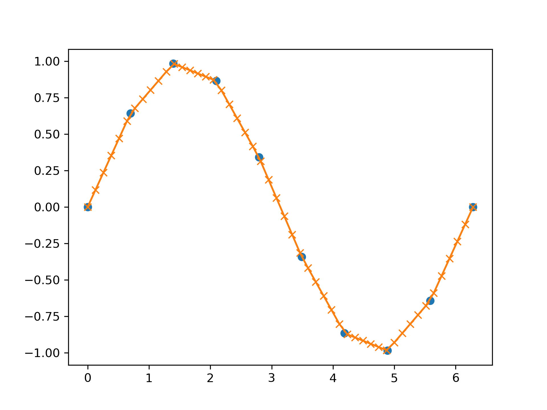
Plot an interpolant to the sine function:

>>> x = np.linspace(0, 2*np.pi, 10)
... y = np.sin(x)
... xvals = np.linspace(0, 2*np.pi, 50)
... yinterp = np.interp(xvals, x, y)
... import matplotlib.pyplot as plt
... plt.plot(x, y, 'o')
[<matplotlib.lines.Line2D object at 0x...>]

>>> plt.plot(xvals, yinterp, '-x')
[<matplotlib.lines.Line2D object at 0x...>]

>>> plt.show()

Interpolation with periodic x-coordinates:

>>> x = [-180, -170, -185, 185, -10, -5, 0, 365]
... xp = [190, -190, 350, -350]
... fp = [5, 10, 3, 4]
... np.interp(x, xp, fp, period=360)
array([7.5 , 5.  , 8.75, 6.25, 3.  , 3.25, 3.5 , 3.75])

Complex interpolation:

>>> x = [1.5, 4.0]
... xp = [2,3,5]
... fp = [1.0j, 0, 2+3j]
... np.interp(x, xp, fp)
array([0.+1.j , 1.+1.5j])

See :

Local connectivity graph

Hover to see nodes names; edges to Self not shown, Caped at 50 nodes.

Using a canvas is more power efficient and can get hundred of nodes ; but does not allow hyperlinks; , arrows or text (beyond on hover)

SVG is more flexible but power hungry; and does not scale well to 50 + nodes.

All aboves nodes referred to, (or are referred from) current nodes; Edges from Self to other have been omitted (or all nodes would be connected to the central node "self" which is not useful). Nodes are colored by the library they belong to, and scaled with the number of references pointing them