lsim(system, U, T, X0=None, interp=True)
If (num, den) is passed in for system
, coefficients for both the numerator and denominator should be specified in descending exponent order (e.g. s^2 + 3s + 5
would be represented as [1, 3, 5]
).
The following gives the number of elements in the tuple and the interpretation:
1: (instance of lti
)
2: (num, den)
3: (zeros, poles, gain)
4: (A, B, C, D)
An input array describing the input at each time T (interpolation is assumed between given times). If there are multiple inputs, then each column of the rank-2 array represents an input. If U = 0 or None, a zero input is used.
The time steps at which the input is defined and at which the output is desired. Must be nonnegative, increasing, and equally spaced.
The initial conditions on the state vector (zero by default).
Whether to use linear (True, the default) or zero-order-hold (False) interpolation for the input array.
Time values for the output.
System response.
Time evolution of the state vector.
Simulate output of a continuous-time linear system.
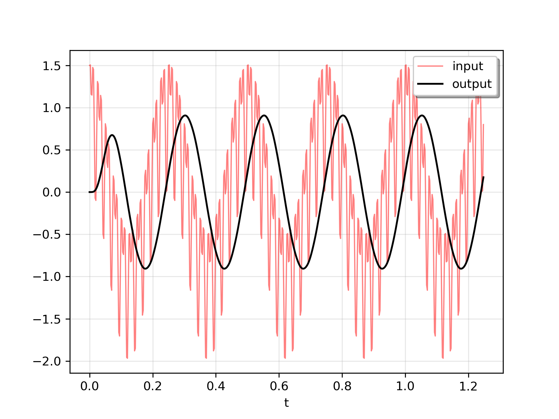
We'll use lsim
to simulate an analog Bessel filter applied to a signal.
>>> from scipy.signal import bessel, lsim
... import matplotlib.pyplot as plt
Create a low-pass Bessel filter with a cutoff of 12 Hz.
>>> b, a = bessel(N=5, Wn=2*np.pi*12, btype='lowpass', analog=True)
Generate data to which the filter is applied.
>>> t = np.linspace(0, 1.25, 500, endpoint=False)
The input signal is the sum of three sinusoidal curves, with frequencies 4 Hz, 40 Hz, and 80 Hz. The filter should mostly eliminate the 40 Hz and 80 Hz components, leaving just the 4 Hz signal.
>>> u = (np.cos(2*np.pi*4*t) + 0.6*np.sin(2*np.pi*40*t) +
...      0.5*np.cos(2*np.pi*80*t))
Simulate the filter with lsim
.
>>> tout, yout, xout = lsim((b, a), U=u, T=t)
Plot the result.
>>> plt.plot(t, u, 'r', alpha=0.5, linewidth=1, label='input')
... plt.plot(tout, yout, 'k', linewidth=1.5, label='output')
... plt.legend(loc='best', shadow=True, framealpha=1)
... plt.grid(alpha=0.3)
... plt.xlabel('t')
... plt.show()
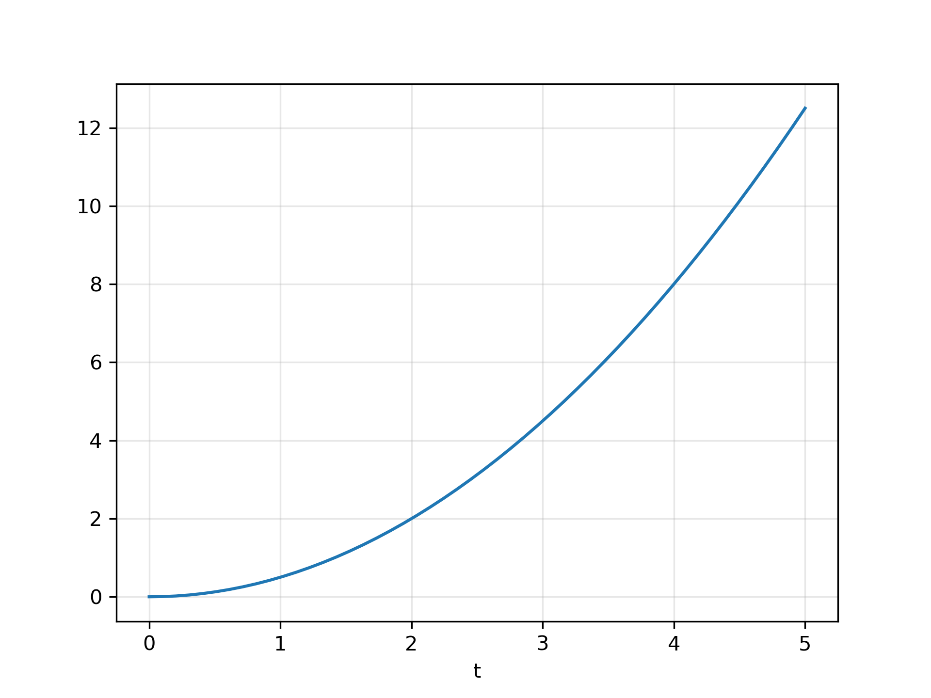
In a second example, we simulate a double integrator y'' = u
, with a constant input u = 1
. We'll use the state space representation of the integrator.
>>> from scipy.signal import lti
... A = np.array([[0.0, 1.0], [0.0, 0.0]])
... B = np.array([[0.0], [1.0]])
... C = np.array([[1.0, 0.0]])
... D = 0.0
... system = lti(A, B, C, D)
t and u define the time and input signal for the system to be simulated.
>>> t = np.linspace(0, 5, num=50)
... u = np.ones_like(t)
Compute the simulation, and then plot y. As expected, the plot shows the curve y = 0.5*t**2
.
>>> tout, y, x = lsim(system, u, t)
... plt.plot(t, y)
... plt.grid(alpha=0.3)
... plt.xlabel('t')
... plt.show()
The following pages refer to to this document either explicitly or contain code examples using this.
scipy.signal._ltisys.lti.output
scipy.signal._ltisys.lsim2
scipy.signal._ltisys.dlsim
scipy.signal._ltisys.lsim
Hover to see nodes names; edges to Self not shown, Caped at 50 nodes.
Using a canvas is more power efficient and can get hundred of nodes ; but does not allow hyperlinks; , arrows or text (beyond on hover)
SVG is more flexible but power hungry; and does not scale well to 50 + nodes.
All aboves nodes referred to, (or are referred from) current nodes; Edges from Self to other have been omitted (or all nodes would be connected to the central node "self" which is not useful). Nodes are colored by the library they belong to, and scaled with the number of references pointing them