dfreqresp(system, w=None, n=10000, whole=False)
If (num, den) is passed in for system
, coefficients for both the numerator and denominator should be specified in descending exponent order (e.g. z^2 + 3z + 5
would be represented as [1, 3, 5]
).
The following gives the number of elements in the tuple and the interpretation:
1 (instance of
dlti)2 (numerator, denominator, dt)
3 (zeros, poles, gain, dt)
4 (A, B, C, D, dt)
Array of frequencies (in radians/sample). Magnitude and phase data is calculated for every value in this array. If not given a reasonable set will be calculated.
Number of frequency points to compute if w is not given. The n frequencies are logarithmically spaced in an interval chosen to include the influence of the poles and zeros of the system.
Normally, if 'w' is not given, frequencies are computed from 0 to the Nyquist frequency, pi radians/sample (upper-half of unit-circle). If :None:None:`whole` is True, compute frequencies from 0 to 2*pi radians/sample.
Calculate the frequency response of a discrete-time system.
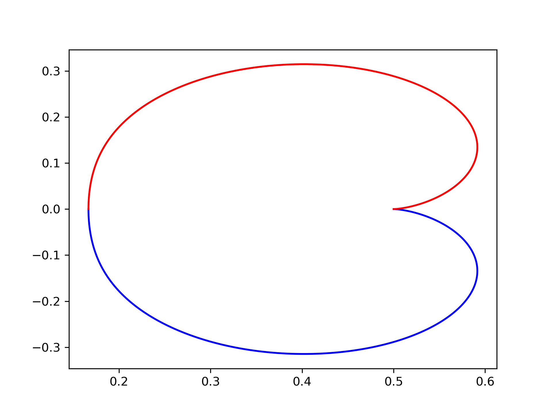
Generating the Nyquist plot of a transfer function
>>> from scipy import signal
... import matplotlib.pyplot as plt
Construct the transfer function $H(z) = \frac{1}{z^2 + 2z + 3}$ with a sampling time of 0.05 seconds:
>>> sys = signal.TransferFunction([1], [1, 2, 3], dt=0.05)
>>> w, H = signal.dfreqresp(sys)
>>> plt.figure()
... plt.plot(H.real, H.imag, "b")
... plt.plot(H.real, -H.imag, "r")
... plt.show()
The following pages refer to to this document either explicitly or contain code examples using this.
scipy.signal._ltisys.dfreqresp
scipy.signal._ltisys.dlti.freqresp
Hover to see nodes names; edges to Self not shown, Caped at 50 nodes.
Using a canvas is more power efficient and can get hundred of nodes ; but does not allow hyperlinks; , arrows or text (beyond on hover)
SVG is more flexible but power hungry; and does not scale well to 50 + nodes.
All aboves nodes referred to, (or are referred from) current nodes; Edges from Self to other have been omitted (or all nodes would be connected to the central node "self" which is not useful). Nodes are colored by the library they belong to, and scaled with the number of references pointing them