bessel(N, Wn, btype='low', analog=False, output='ba', norm='phase', fs=None)
Design an Nth-order digital or analog Bessel filter and return the filter coefficients.
Also known as a Thomson filter, the analog Bessel filter has maximally flat group delay and maximally linear phase response, with very little ringing in the step response.
The Bessel is inherently an analog filter. This function generates digital Bessel filters using the bilinear transform, which does not preserve the phase response of the analog filter. As such, it is only approximately correct at frequencies below about fs/4. To get maximally-flat group delay at higher frequencies, the analog Bessel filter must be transformed using phase-preserving techniques.
See besselap
for implementation details and references.
The 'sos'
output parameter was added in 0.16.0.
The order of the filter.
A scalar or length-2 sequence giving the critical frequencies (defined by the :None:None:`norm` parameter). For analog filters, :None:None:`Wn` is an angular frequency (e.g., rad/s).
For digital filters, :None:None:`Wn` are in the same units as :None:None:`fs`. By default, :None:None:`fs` is 2 half-cycles/sample, so these are normalized from 0 to 1, where 1 is the Nyquist frequency. (:None:None:`Wn` is thus in half-cycles / sample.)
The type of filter. Default is 'lowpass'.
When True, return an analog filter, otherwise a digital filter is returned. (See Notes.)
Type of output: numerator/denominator ('ba'), pole-zero ('zpk'), or second-order sections ('sos'). Default is 'ba'.
Critical frequency normalization:
phase
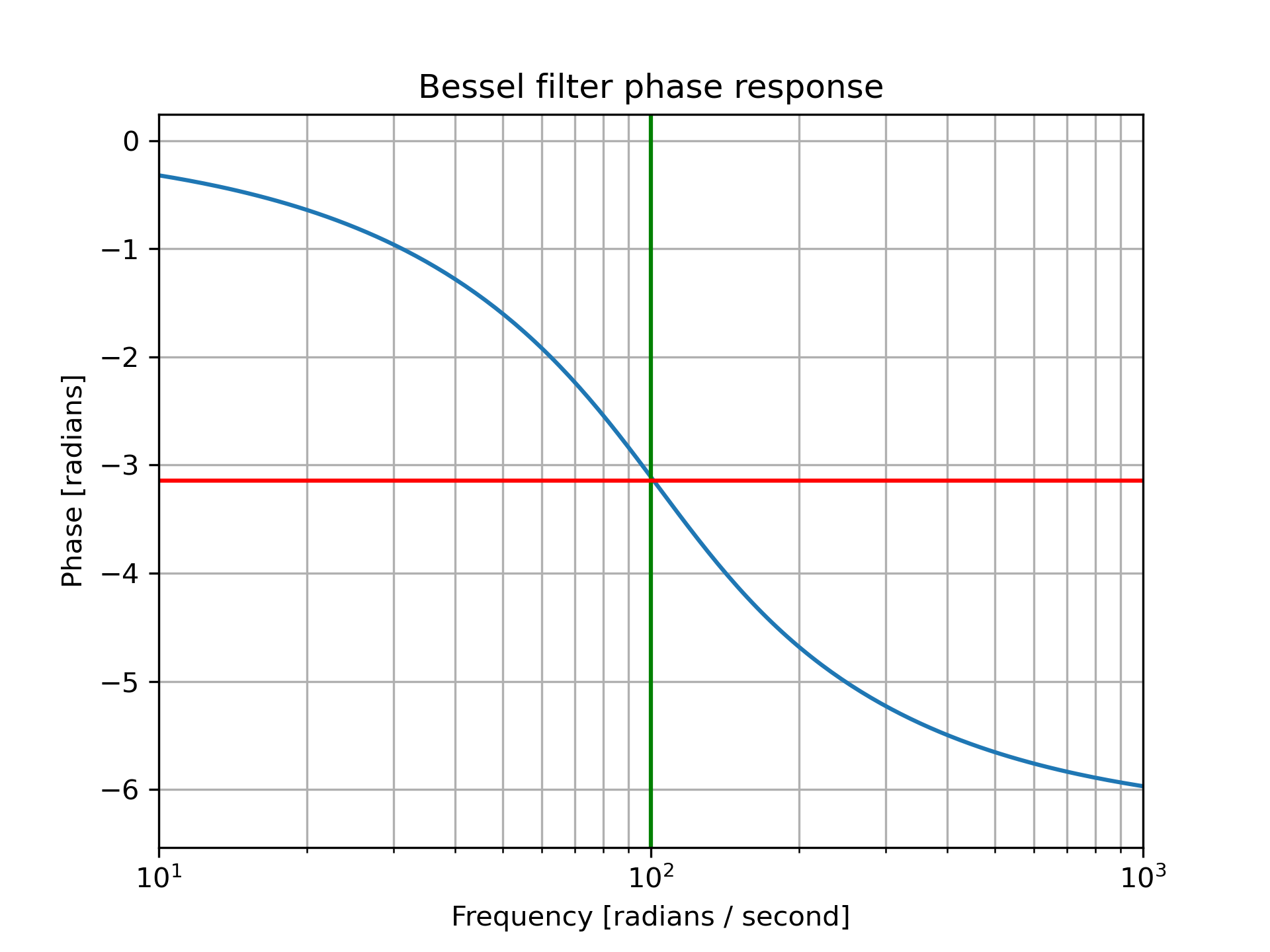
The filter is normalized such that the phase response reaches its midpoint at angular (e.g. rad/s) frequency :None:None:`Wn`. This happens for both low-pass and high-pass filters, so this is the "phase-matched" case.
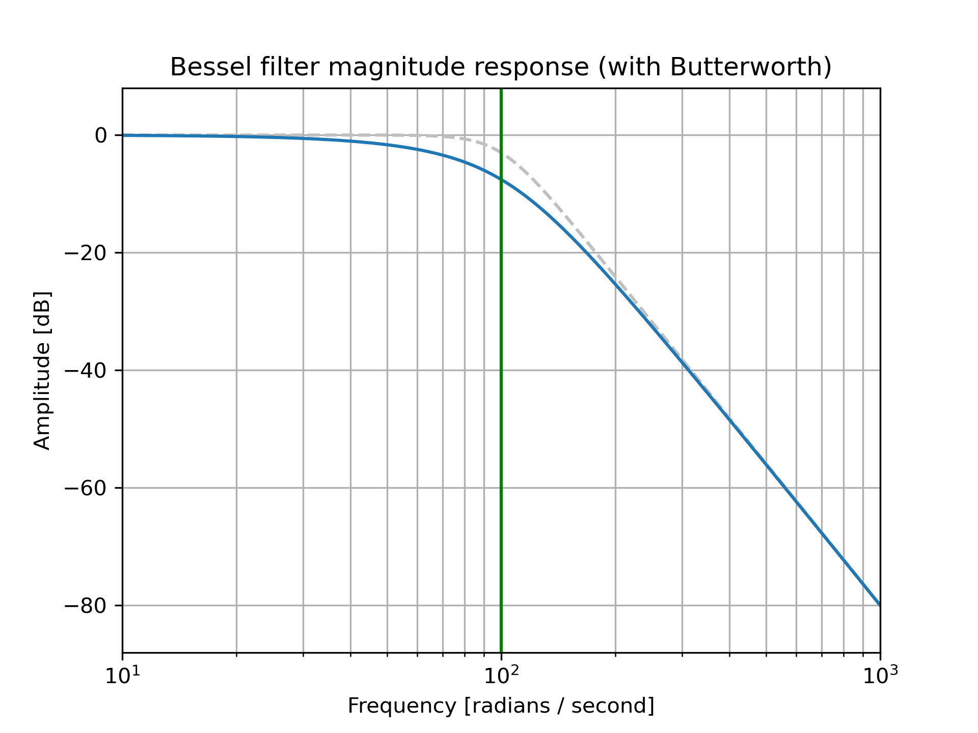
The magnitude response asymptotes are the same as a Butterworth filter of the same order with a cutoff of :None:None:`Wn`.
This is the default, and matches MATLAB's implementation.
delay
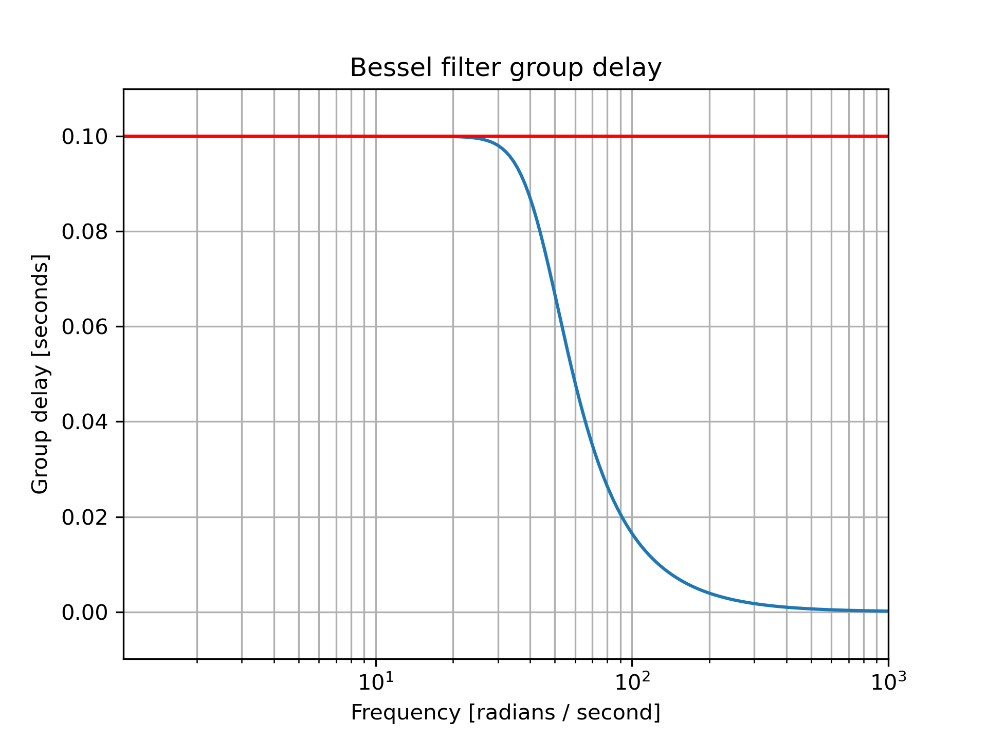
The filter is normalized such that the group delay in the passband is 1/:None:None:`Wn` (e.g., seconds). This is the "natural" type obtained by solving Bessel polynomials.
mag
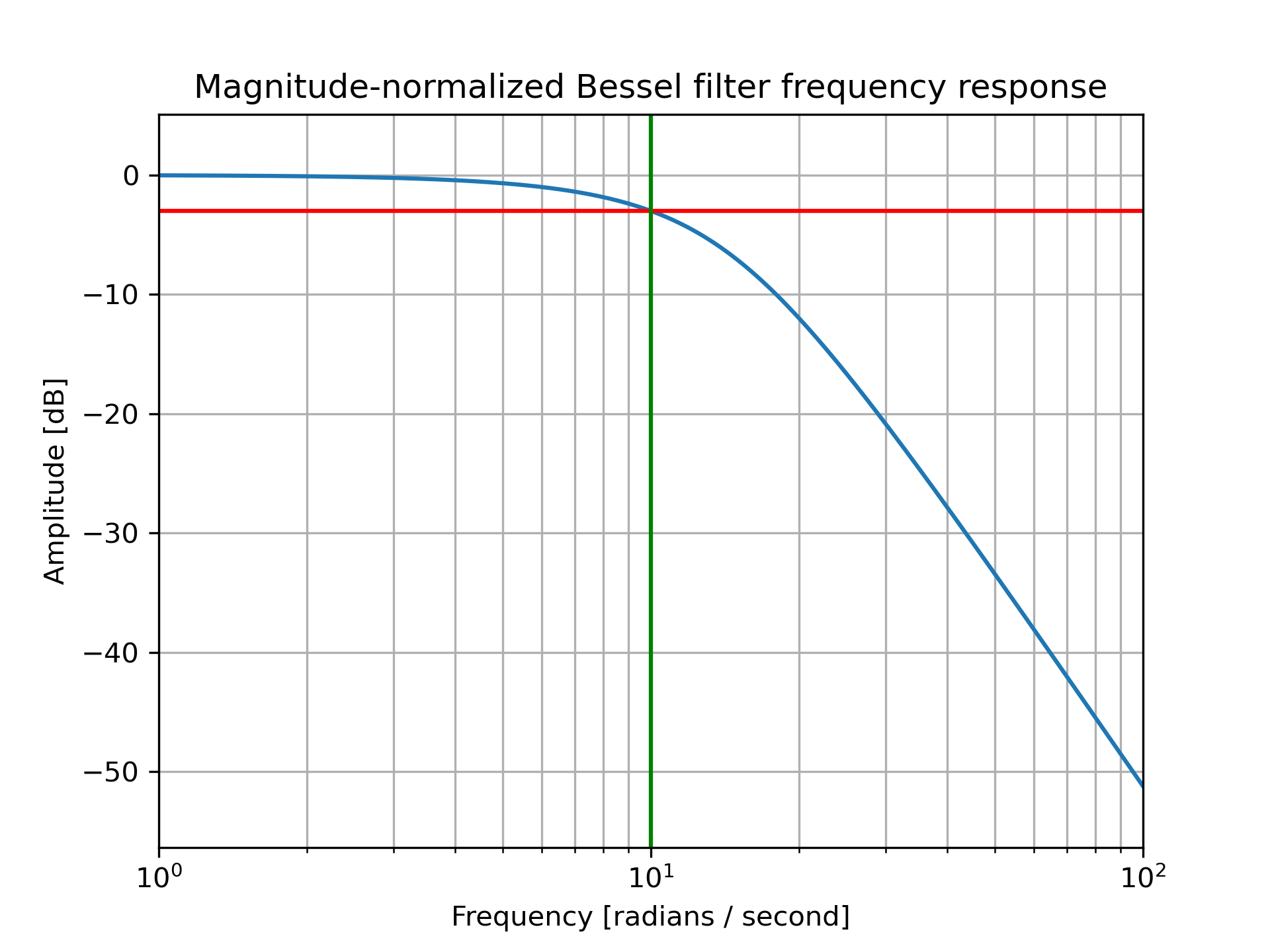
The filter is normalized such that the gain magnitude is -3 dB at angular frequency :None:None:`Wn`.
The sampling frequency of the digital system.
Numerator (b) and denominator (a) polynomials of the IIR filter. Only returned if output='ba'
.
Zeros, poles, and system gain of the IIR filter transfer function. Only returned if output='zpk'
.
Second-order sections representation of the IIR filter. Only returned if output=='sos'
.
Bessel/Thomson digital and analog filter design.
Plot the phase-normalized frequency response, showing the relationship to the Butterworth's cutoff frequency (green):
>>> from scipy import signal
... import matplotlib.pyplot as plt
>>> b, a = signal.butter(4, 100, 'low', analog=True)
... w, h = signal.freqs(b, a)
... plt.semilogx(w, 20 * np.log10(np.abs(h)), color='silver', ls='dashed')
... b, a = signal.bessel(4, 100, 'low', analog=True, norm='phase')
... w, h = signal.freqs(b, a)
... plt.semilogx(w, 20 * np.log10(np.abs(h)))
... plt.title('Bessel filter magnitude response (with Butterworth)')
... plt.xlabel('Frequency [radians / second]')
... plt.ylabel('Amplitude [dB]')
... plt.margins(0, 0.1)
... plt.grid(which='both', axis='both')
... plt.axvline(100, color='green')  # cutoff frequency
... plt.show()
and the phase midpoint:
>>> plt.figure()
... plt.semilogx(w, np.unwrap(np.angle(h)))
... plt.axvline(100, color='green')  # cutoff frequency
... plt.axhline(-np.pi, color='red')  # phase midpoint
... plt.title('Bessel filter phase response')
... plt.xlabel('Frequency [radians / second]')
... plt.ylabel('Phase [radians]')
... plt.margins(0, 0.1)
... plt.grid(which='both', axis='both')
... plt.show()
Plot the magnitude-normalized frequency response, showing the -3 dB cutoff:
>>> b, a = signal.bessel(3, 10, 'low', analog=True, norm='mag')
... w, h = signal.freqs(b, a)
... plt.semilogx(w, 20 * np.log10(np.abs(h)))
... plt.axhline(-3, color='red')  # -3 dB magnitude
... plt.axvline(10, color='green')  # cutoff frequency
... plt.title('Magnitude-normalized Bessel filter frequency response')
... plt.xlabel('Frequency [radians / second]')
... plt.ylabel('Amplitude [dB]')
... plt.margins(0, 0.1)
... plt.grid(which='both', axis='both')
... plt.show()
Plot the delay-normalized filter, showing the maximally-flat group delay at 0.1 seconds:
>>> b, a = signal.bessel(5, 1/0.1, 'low', analog=True, norm='delay')
... w, h = signal.freqs(b, a)
... plt.figure()
... plt.semilogx(w[1:], -np.diff(np.unwrap(np.angle(h)))/np.diff(w))
... plt.axhline(0.1, color='red')  # 0.1 seconds group delay
... plt.title('Bessel filter group delay')
... plt.xlabel('Frequency [radians / second]')
... plt.ylabel('Group delay [seconds]')
... plt.margins(0, 0.1)
... plt.grid(which='both', axis='both')
... plt.show()
The following pages refer to to this document either explicitly or contain code examples using this.
scipy.signal._ltisys.lsim
scipy.signal._ltisys.lsim2
scipy.signal._filter_design.iirfilter
scipy.signal._filter_design.besselap
scipy.signal._filter_design.bessel
scipy.signal._filter_design.iirdesign
Hover to see nodes names; edges to Self not shown, Caped at 50 nodes.
Using a canvas is more power efficient and can get hundred of nodes ; but does not allow hyperlinks; , arrows or text (beyond on hover)
SVG is more flexible but power hungry; and does not scale well to 50 + nodes.
All aboves nodes referred to, (or are referred from) current nodes; Edges from Self to other have been omitted (or all nodes would be connected to the central node "self" which is not useful). Nodes are colored by the library they belong to, and scaled with the number of references pointing them