butter(N, Wn, btype='low', analog=False, output='ba', fs=None)
Design an Nth-order digital or analog Butterworth filter and return the filter coefficients.
The Butterworth filter has maximally flat frequency response in the passband.
The 'sos'
output parameter was added in 0.16.0.
If the transfer function form [b, a]
is requested, numerical problems can occur since the conversion between roots and the polynomial coefficients is a numerically sensitive operation, even for N >= 4. It is recommended to work with the SOS representation.
The order of the filter.
The critical frequency or frequencies. For lowpass and highpass filters, Wn is a scalar; for bandpass and bandstop filters, Wn is a length-2 sequence.
For a Butterworth filter, this is the point at which the gain drops to 1/sqrt(2) that of the passband (the "-3 dB point").
For digital filters, if :None:None:`fs` is not specified, :None:None:`Wn` units are normalized from 0 to 1, where 1 is the Nyquist frequency (:None:None:`Wn` is thus in half cycles / sample and defined as 2*critical frequencies / :None:None:`fs`). If :None:None:`fs` is specified, :None:None:`Wn` is in the same units as :None:None:`fs`.
For analog filters, :None:None:`Wn` is an angular frequency (e.g. rad/s).
The type of filter. Default is 'lowpass'.
When True, return an analog filter, otherwise a digital filter is returned.
Type of output: numerator/denominator ('ba'), pole-zero ('zpk'), or second-order sections ('sos'). Default is 'ba' for backwards compatibility, but 'sos' should be used for general-purpose filtering.
The sampling frequency of the digital system.
Numerator (b) and denominator (a) polynomials of the IIR filter. Only returned if output='ba'
.
Zeros, poles, and system gain of the IIR filter transfer function. Only returned if output='zpk'
.
Second-order sections representation of the IIR filter. Only returned if output=='sos'
.
Butterworth digital and analog filter design.
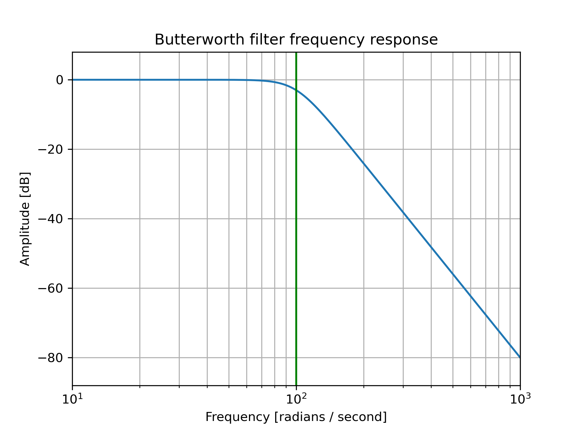
Design an analog filter and plot its frequency response, showing the critical points:
>>> from scipy import signal
... import matplotlib.pyplot as plt
>>> b, a = signal.butter(4, 100, 'low', analog=True)
... w, h = signal.freqs(b, a)
... plt.semilogx(w, 20 * np.log10(abs(h)))
... plt.title('Butterworth filter frequency response')
... plt.xlabel('Frequency [radians / second]')
... plt.ylabel('Amplitude [dB]')
... plt.margins(0, 0.1)
... plt.grid(which='both', axis='both')
... plt.axvline(100, color='green') # cutoff frequency
... plt.show()
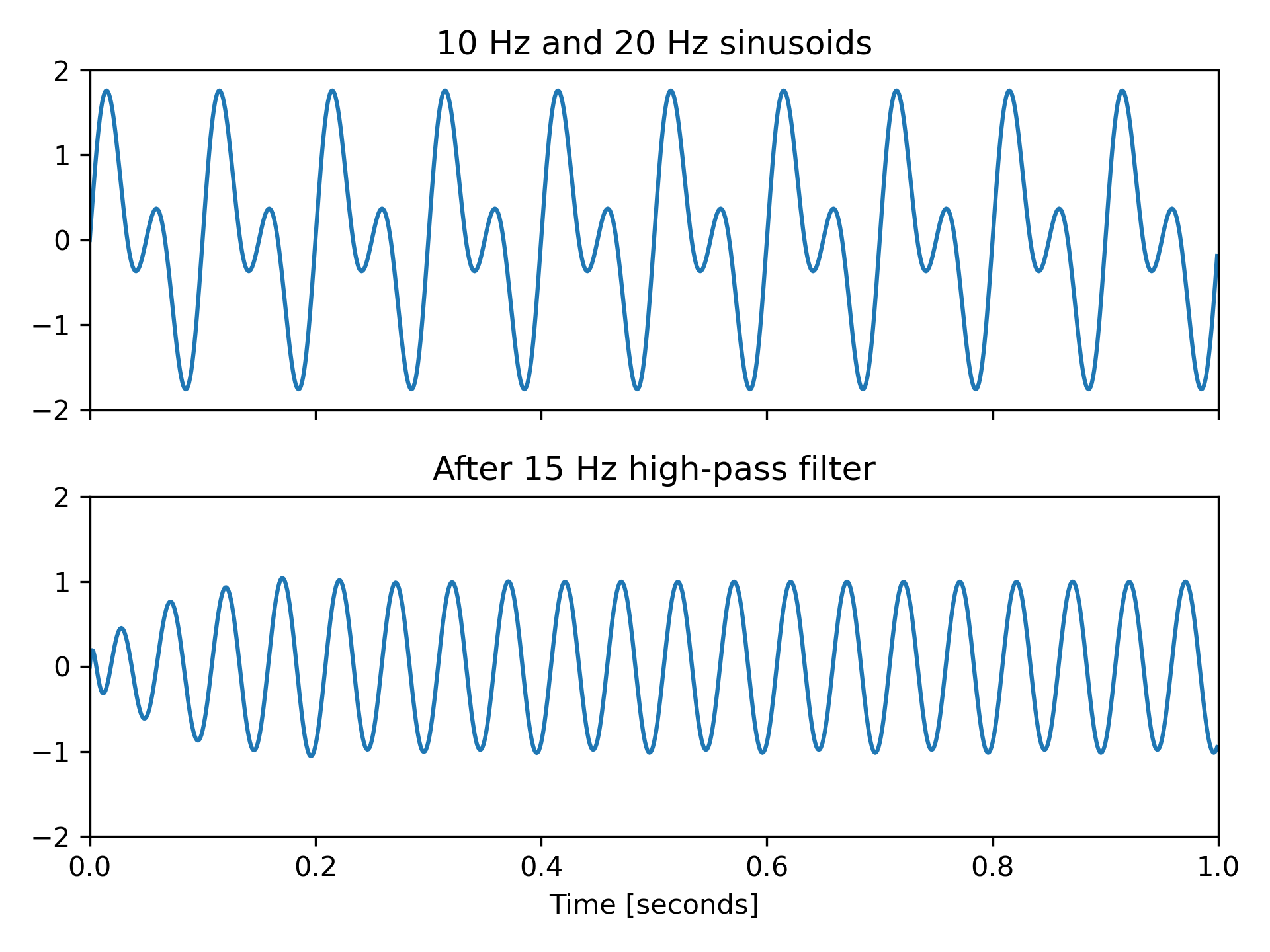
Generate a signal made up of 10 Hz and 20 Hz, sampled at 1 kHz
>>> t = np.linspace(0, 1, 1000, False)  # 1 second
... sig = np.sin(2*np.pi*10*t) + np.sin(2*np.pi*20*t)
... fig, (ax1, ax2) = plt.subplots(2, 1, sharex=True)
... ax1.plot(t, sig)
... ax1.set_title('10 Hz and 20 Hz sinusoids')
... ax1.axis([0, 1, -2, 2])
Design a digital high-pass filter at 15 Hz to remove the 10 Hz tone, and apply it to the signal. (It's recommended to use second-order sections format when filtering, to avoid numerical error with transfer function ( ba
) format):
>>> sos = signal.butter(10, 15, 'hp', fs=1000, output='sos')
... filtered = signal.sosfilt(sos, sig)
... ax2.plot(t, filtered)
... ax2.set_title('After 15 Hz high-pass filter')
... ax2.axis([0, 1, -2, 2])
... ax2.set_xlabel('Time [seconds]')
... plt.tight_layout()
... plt.show()
The following pages refer to to this document either explicitly or contain code examples using this.
scipy.signal._filter_design.iirfilter
scipy.signal._signaltools.sosfilt_zi
scipy.signal._ltisys.dimpulse
scipy.signal._ltisys.dstep
scipy.signal._filter_design.ellip
scipy.signal._signaltools.filtfilt
scipy.signal._signaltools.lfilter_zi
scipy.signal._filter_design.butter
scipy.signal._spectral_py.coherence
scipy.signal._signaltools.sosfiltfilt
scipy.signal._spectral_py.csd
scipy.signal._signaltools.lfilter
scipy.signal._filter_design.buttap
scipy.signal._waveforms.unit_impulse
scipy.signal._filter_design.freqz_zpk
scipy.signal._filter_design.bessel
scipy.signal._filter_design.bilinear
scipy.signal._filter_design.iirdesign
scipy.signal._filter_design.buttord
scipy.signal._filter_design.bilinear_zpk
Hover to see nodes names; edges to Self not shown, Caped at 50 nodes.
Using a canvas is more power efficient and can get hundred of nodes ; but does not allow hyperlinks; , arrows or text (beyond on hover)
SVG is more flexible but power hungry; and does not scale well to 50 + nodes.
All aboves nodes referred to, (or are referred from) current nodes; Edges from Self to other have been omitted (or all nodes would be connected to the central node "self" which is not useful). Nodes are colored by the library they belong to, and scaled with the number of references pointing them