Document

scipy 1.8.0 Pypi GitHub Homepage

Other Docs

Notes Parameters Returns BackRef

sosfiltfilt(sos, x, axis=-1, padtype='odd', padlen=None)

See filtfilt for more complete information about this method.

Notes

versionadded

Parameters

sos : array_like

Array of second-order filter coefficients, must have shape (n_sections, 6) . Each row corresponds to a second-order section, with the first three columns providing the numerator coefficients and the last three providing the denominator coefficients.

x : array_like

The array of data to be filtered.

axis : int, optional

The axis of x to which the filter is applied. Default is -1.

padtype : str or None, optional

Must be 'odd', 'even', 'constant', or None. This determines the type of extension to use for the padded signal to which the filter is applied. If :None:None:`padtype` is None, no padding is used. The default is 'odd'.

padlen : int or None, optional

The number of elements by which to extend x at both ends of :None:None:`axis` before applying the filter. This value must be less than x.shape[axis] - 1 . padlen=0 implies no padding. The default value is:

3 * (2 * len(sos) + 1 - min((sos[:, 2] == 0).sum(),
                            (sos[:, 5] == 0).sum()))

The extra subtraction at the end attempts to compensate for poles and zeros at the origin (e.g. for odd-order filters) to yield equivalent estimates of :None:None:`padlen` to those of filtfilt for second-order section filters built with scipy.signal functions.

Returns

y : ndarray: The filtered output with the same shape as x.

A forward-backward digital filter using cascaded second-order sections.

Examples

>>> from scipy.signal import sosfiltfilt, butter
... import matplotlib.pyplot as plt
... rng = np.random.default_rng()

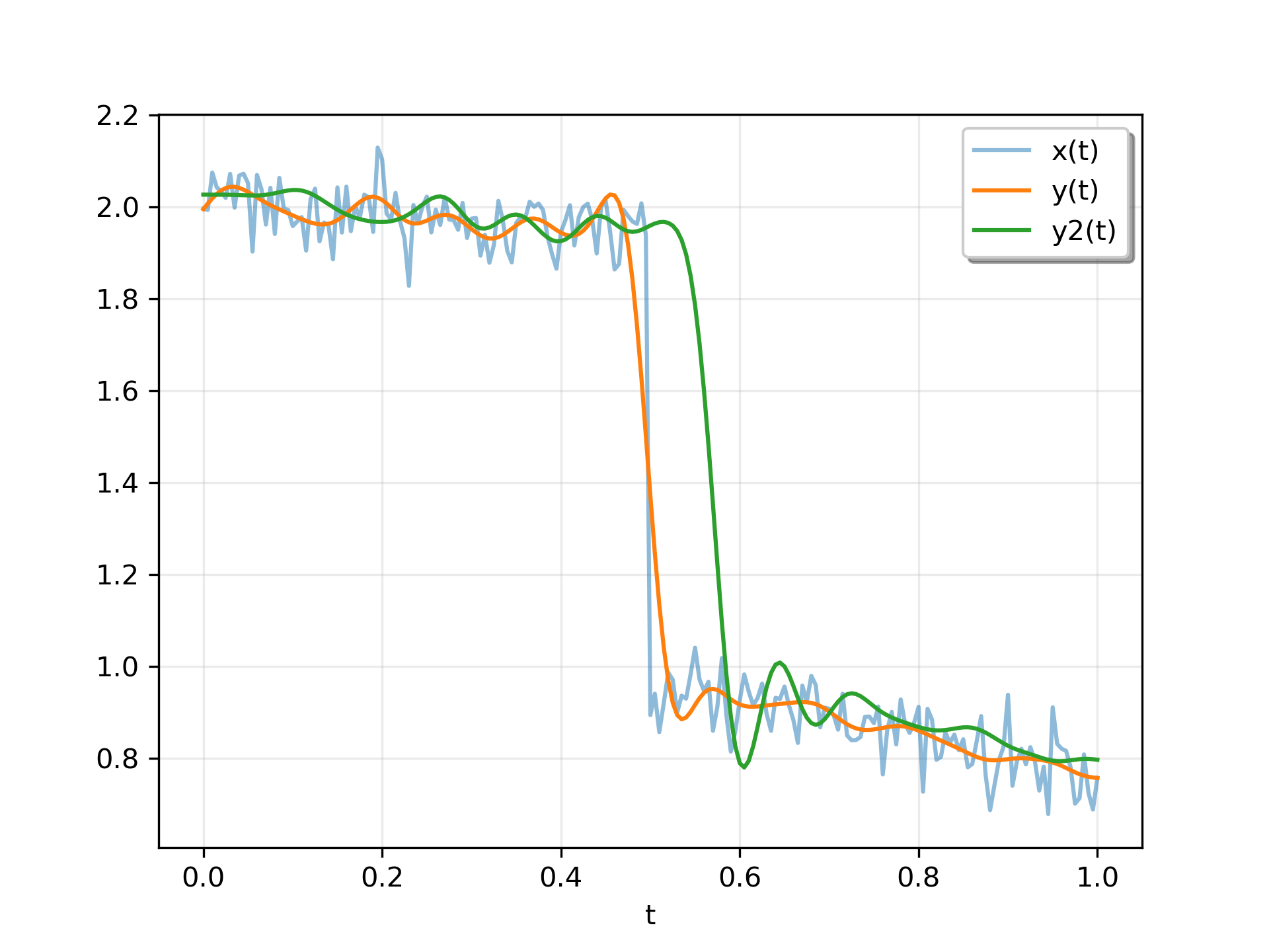
Create an interesting signal to filter.

>>> n = 201
... t = np.linspace(0, 1, n)
... x = 1 + (t < 0.5) - 0.25*t**2 + 0.05*rng.standard_normal(n)

Create a lowpass Butterworth filter, and use it to filter x.

>>> sos = butter(4, 0.125, output='sos')
... y = sosfiltfilt(sos, x)

For comparison, apply an 8th order filter using sosfilt . The filter is initialized using the mean of the first four values of x.

>>> from scipy.signal import sosfilt, sosfilt_zi
... sos8 = butter(8, 0.125, output='sos')
... zi = x[:4].mean() * sosfilt_zi(sos8)
... y2, zo = sosfilt(sos8, x, zi=zi)

Plot the results. Note that the phase of y matches the input, while y2 has a significant phase delay.

>>> plt.plot(t, x, alpha=0.5, label='x(t)')
... plt.plot(t, y, label='y(t)')
... plt.plot(t, y2, label='y2(t)')
... plt.legend(framealpha=1, shadow=True)
... plt.grid(alpha=0.25)
... plt.xlabel('t')
... plt.show()

See :

Back References

The following pages refer to to this document either explicitly or contain code examples using this.

scipy.signal._signaltools.sosfilt scipy.signal._signaltools.lfilter scipy.signal._signaltools.sosfiltfilt scipy.signal._signaltools.filtfilt

Local connectivity graph

Hover to see nodes names; edges to Self not shown, Caped at 50 nodes.

Using a canvas is more power efficient and can get hundred of nodes ; but does not allow hyperlinks; , arrows or text (beyond on hover)

SVG is more flexible but power hungry; and does not scale well to 50 + nodes.

All aboves nodes referred to, (or are referred from) current nodes; Edges from Self to other have been omitted (or all nodes would be connected to the central node "self" which is not useful). Nodes are colored by the library they belong to, and scaled with the number of references pointing them