correlate(in1, in2, mode='full', method='auto')
Cross-correlate :None:None:`in1` and in2
, with the output size determined by the :None:None:`mode` argument.
The correlation z of two d-dimensional arrays x and y is defined as:
z[...,k,...] = sum[..., i_l, ...] x[..., i_l,...] * conj(y[..., i_l - k,...])
This way, if x and y are 1-D arrays and z = correlate(x, y, 'full')
then
for $k = 0, 1, ..., ||x|| + ||y|| - 2$
where $||x||$
is the length of x
, $N = \max(||x||,||y||)$
, and $y_m$
is 0 when m is outside the range of y.
method='fft'
only works for numerical arrays as it relies on fftconvolve
. In certain cases (i.e., arrays of objects or when rounding integers can lose precision), method='direct'
is always used.
When using "same" mode with even-length inputs, the outputs of correlate
and correlate2d
differ: There is a 1-index offset between them.
First input.
Second input. Should have the same number of dimensions as :None:None:`in1`.
A string indicating the size of the output:
full
The output is the full discrete linear cross-correlation of the inputs. (Default)
valid
The output consists only of those elements that do not rely on the zero-padding. In 'valid' mode, either :None:None:`in1` or in2
must be at least as large as the other in every dimension.
same
The output is the same size as :None:None:`in1`, centered with respect to the 'full' output.
A string indicating which method to use to calculate the correlation.
direct
The correlation is determined directly from sums, the definition of correlation.
fft
The Fast Fourier Transform is used to perform the correlation more quickly (only available for numerical arrays.)
auto
Automatically chooses direct or Fourier method based on an estimate of which is faster (default). See convolve
Notes for more detail.
An N-dimensional array containing a subset of the discrete linear cross-correlation of :None:None:`in1` with in2
.
Cross-correlate two N-dimensional arrays.
choose_conv_method
contains more documentation on :None:None:`method`.
correlation_lags
calculates the lag / displacement indices array for 1D cross-correlation.
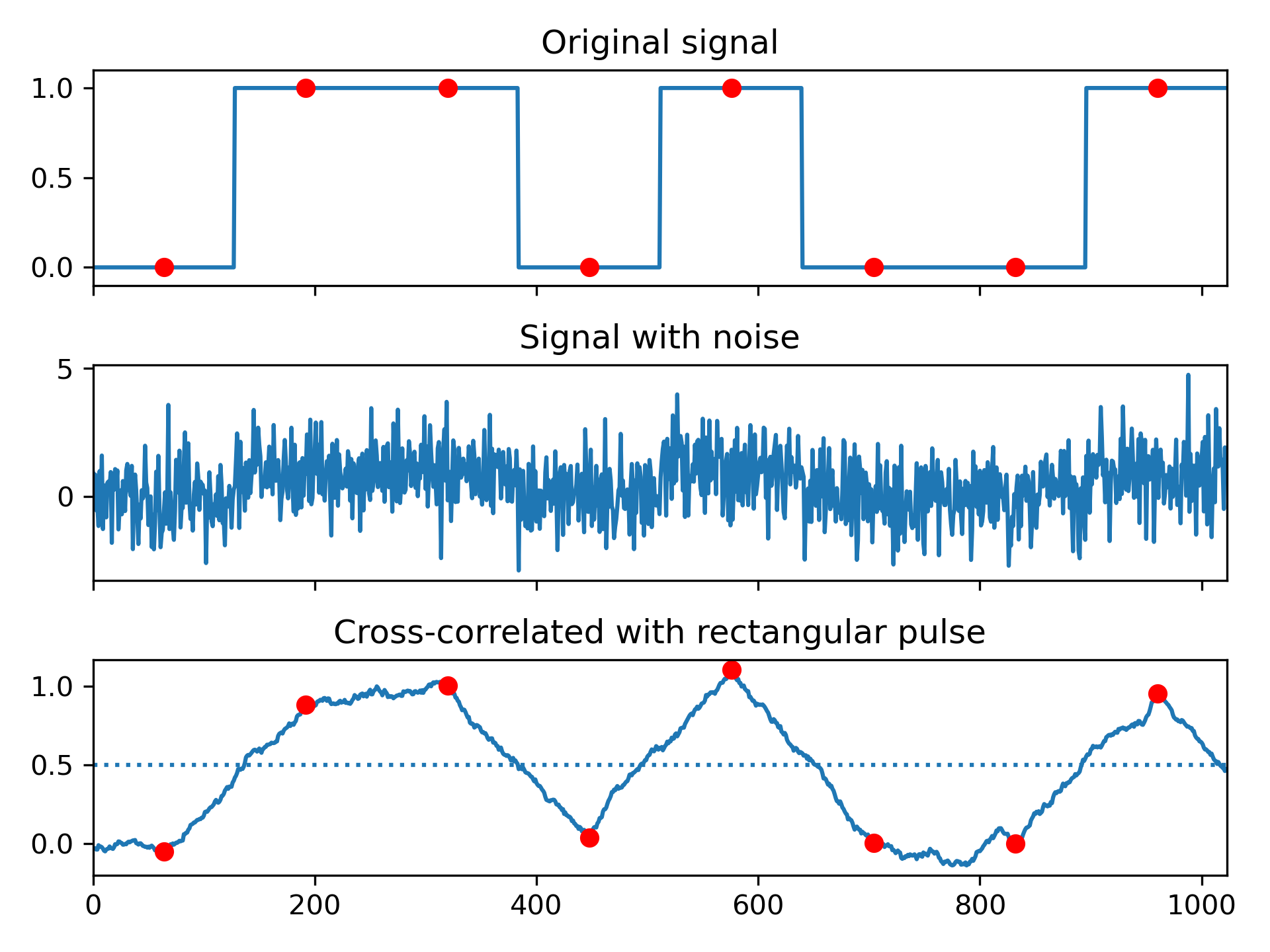
Implement a matched filter using cross-correlation, to recover a signal that has passed through a noisy channel.
>>> from scipy import signal
... import matplotlib.pyplot as plt
... rng = np.random.default_rng()
>>> sig = np.repeat([0., 1., 1., 0., 1., 0., 0., 1.], 128)
... sig_noise = sig + rng.standard_normal(len(sig))
... corr = signal.correlate(sig_noise, np.ones(128), mode='same') / 128
>>> clock = np.arange(64, len(sig), 128)
... fig, (ax_orig, ax_noise, ax_corr) = plt.subplots(3, 1, sharex=True)
... ax_orig.plot(sig)
... ax_orig.plot(clock, sig[clock], 'ro')
... ax_orig.set_title('Original signal')
... ax_noise.plot(sig_noise)
... ax_noise.set_title('Signal with noise')
... ax_corr.plot(corr)
... ax_corr.plot(clock, corr[clock], 'ro')
... ax_corr.axhline(0.5, ls=':')
... ax_corr.set_title('Cross-correlated with rectangular pulse')
... ax_orig.margins(0, 0.1)
... fig.tight_layout()
... plt.show()
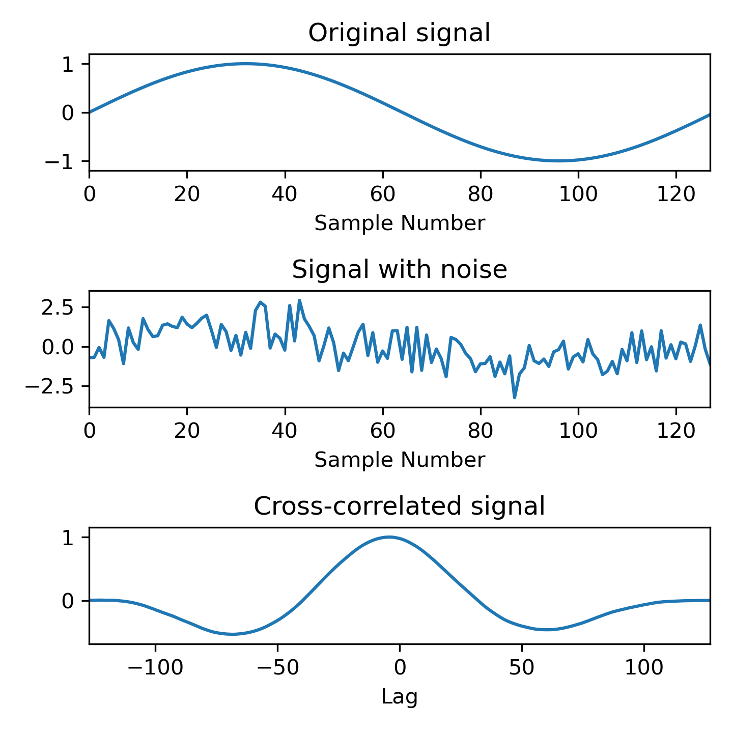
Compute the cross-correlation of a noisy signal with the original signal.
>>> x = np.arange(128) / 128
... sig = np.sin(2 * np.pi * x)
... sig_noise = sig + rng.standard_normal(len(sig))
... corr = signal.correlate(sig_noise, sig)
... lags = signal.correlation_lags(len(sig), len(sig_noise))
... corr /= np.max(corr)
>>> fig, (ax_orig, ax_noise, ax_corr) = plt.subplots(3, 1, figsize=(4.8, 4.8))
... ax_orig.plot(sig)
... ax_orig.set_title('Original signal')
... ax_orig.set_xlabel('Sample Number')
... ax_noise.plot(sig_noise)
... ax_noise.set_title('Signal with noise')
... ax_noise.set_xlabel('Sample Number')
... ax_corr.plot(lags, corr)
... ax_corr.set_title('Cross-correlated signal')
... ax_corr.set_xlabel('Lag')
... ax_orig.margins(0, 0.1)
... ax_noise.margins(0, 0.1)
... ax_corr.margins(0, 0.1)
... fig.tight_layout()
... plt.show()
The following pages refer to to this document either explicitly or contain code examples using this.
numpy.correlate
scipy.signal._signaltools.correlation_lags
scipy.signal._signaltools.choose_conv_method
scipy.signal._signaltools.convolve
scipy.signal._signaltools.correlate2d
scipy.signal._signaltools.correlate
Hover to see nodes names; edges to Self not shown, Caped at 50 nodes.
Using a canvas is more power efficient and can get hundred of nodes ; but does not allow hyperlinks; , arrows or text (beyond on hover)
SVG is more flexible but power hungry; and does not scale well to 50 + nodes.
All aboves nodes referred to, (or are referred from) current nodes; Edges from Self to other have been omitted (or all nodes would be connected to the central node "self" which is not useful). Nodes are colored by the library they belong to, and scaled with the number of references pointing them