lfilter(b, a, x, axis=-1, zi=None)
Filter a data sequence, x, using a digital filter. This works for many fundamental data types (including Object type). The filter is a direct form II transposed implementation of the standard difference equation (see Notes).
The function sosfilt
(and filter design using output='sos'
) should be preferred over lfilter
for most filtering tasks, as second-order sections have fewer numerical problems.
The filter function is implemented as a direct II transposed structure. This means that the filter implements:
a[0]*y[n] = b[0]*x[n] + b[1]*x[n-1] + ... + b[M]*x[n-M]
                      - a[1]*y[n-1] - ... - a[N]*y[n-N]
where :None:None:`M` is the degree of the numerator, :None:None:`N` is the degree of the denominator, and :None:None:`n` is the sample number. It is implemented using the following difference equations (assuming M = N):
a[0]*y[n] = b[0] * x[n]               + d[0][n-1]
  d[0][n] = b[1] * x[n] - a[1] * y[n] + d[1][n-1]
  d[1][n] = b[2] * x[n] - a[2] * y[n] + d[2][n-1]
...
d[N-2][n] = b[N-1]*x[n] - a[N-1]*y[n] + d[N-1][n-1]
d[N-1][n] = b[N] * x[n] - a[N] * y[n]
where d
are the state variables.
The rational transfer function describing this filter in the z-transform domain is:
                    -1              -M
        b[0] + b[1]z  + ... + b[M] z
Y(z) = -------------------------------- X(z)
                    -1              -N
        a[0] + a[1]z  + ... + a[N] z
The numerator coefficient vector in a 1-D sequence.
The denominator coefficient vector in a 1-D sequence. If a[0]
is not 1, then both a and b are normalized by a[0]
.
An N-dimensional input array.
The axis of the input data array along which to apply the linear filter. The filter is applied to each subarray along this axis. Default is -1.
Initial conditions for the filter delays. It is a vector (or array of vectors for an N-dimensional input) of length max(len(a), len(b)) - 1
. If :None:None:`zi` is None or is not given then initial rest is assumed. See lfiltic
for more information.
The output of the digital filter.
If :None:None:`zi` is None, this is not returned, otherwise, :None:None:`zf` holds the final filter delay values.
Filter data along one-dimension with an IIR or FIR filter.
filtfilt
A forward-backward filter, to obtain a filter with linear phase.
lfilter_zi
Compute initial state (steady state of step response) for :None:None:`lfilter`.
lfiltic
Construct initial conditions for :None:None:`lfilter`.
savgol_filter
A Savitzky-Golay filter.
sosfilt
Filter data using cascaded second-order sections.
sosfiltfilt
A forward-backward filter using second-order sections.
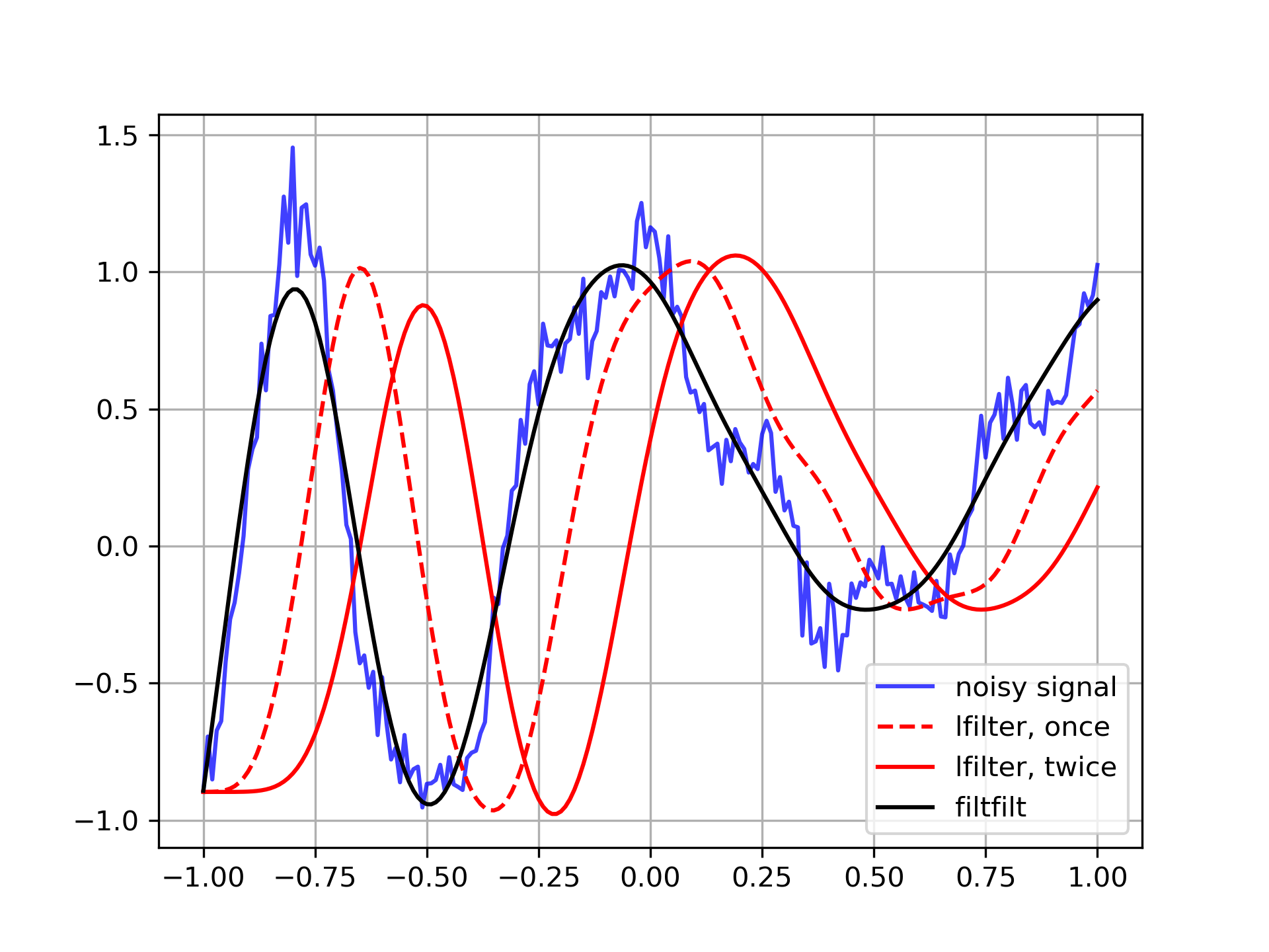
Generate a noisy signal to be filtered:
>>> from scipy import signal
... import matplotlib.pyplot as plt
... rng = np.random.default_rng()
... t = np.linspace(-1, 1, 201)
... x = (np.sin(2*np.pi*0.75*t*(1-t) + 2.1) +
...      0.1*np.sin(2*np.pi*1.25*t + 1) +
...      0.18*np.cos(2*np.pi*3.85*t))
... xn = x + rng.standard_normal(len(t)) * 0.08
Create an order 3 lowpass butterworth filter:
>>> b, a = signal.butter(3, 0.05)
Apply the filter to xn. Use lfilter_zi to choose the initial condition of the filter:
>>> zi = signal.lfilter_zi(b, a)
... z, _ = signal.lfilter(b, a, xn, zi=zi*xn[0])
Apply the filter again, to have a result filtered at an order the same as filtfilt:
>>> z2, _ = signal.lfilter(b, a, z, zi=zi*z[0])
Use filtfilt to apply the filter:
>>> y = signal.filtfilt(b, a, xn)
Plot the original signal and the various filtered versions:
>>> plt.figure
... plt.plot(t, xn, 'b', alpha=0.75)
... plt.plot(t, z, 'r--', t, z2, 'r', t, y, 'k')
... plt.legend(('noisy signal', 'lfilter, once', 'lfilter, twice',
...             'filtfilt'), loc='best')
... plt.grid(True)
... plt.show()
The following pages refer to to this document either explicitly or contain code examples using this.
scipy.signal._spectral_py.coherence
scipy.signal._signaltools.lfilter_zi
scipy.signal._signaltools.lfilter
scipy.signal._spectral_py.csd
scipy.signal._waveforms.unit_impulse
scipy.signal._signaltools.filtfilt
scipy.signal._signaltools.lfiltic
scipy.signal._signaltools.decimate
scipy.signal._signaltools.sosfilt
Hover to see nodes names; edges to Self not shown, Caped at 50 nodes.
Using a canvas is more power efficient and can get hundred of nodes ; but does not allow hyperlinks; , arrows or text (beyond on hover)
SVG is more flexible but power hungry; and does not scale well to 50 + nodes.
All aboves nodes referred to, (or are referred from) current nodes; Edges from Self to other have been omitted (or all nodes would be connected to the central node "self" which is not useful). Nodes are colored by the library they belong to, and scaled with the number of references pointing them