freqz(b, a=1, worN=512, whole=False, plot=None, fs=6.283185307179586, include_nyquist=False)
Given the M-order numerator b and N-order denominator a of a digital filter, compute its frequency response:
            jw                 -jw              -jwM
   jw    B(e  )    b[0] + b[1]e    + ... + b[M]e
H(e  ) = ------ = -----------------------------------
            jw                 -jw              -jwN
         A(e  )    a[0] + a[1]e    + ... + a[N]e
Using Matplotlib's matplotlib.pyplot.plot
function as the callable for :None:None:`plot` produces unexpected results, as this plots the real part of the complex transfer function, not the magnitude. Try lambda w, h: plot(w, np.abs(h))
.
A direct computation via (R)FFT is used to compute the frequency response when the following conditions are met:
An integer value is given for :None:None:`worN`.
:None:None:`worN` is fast to compute via FFT (i.e., :None:None:`next_fast_len(worN) <scipy.fft.next_fast_len>` equals :None:None:`worN`).
The denominator coefficients are a single value ( a.shape[0] == 1
).
:None:None:`worN` is at least as long as the numerator coefficients ( worN >= b.shape[0]
).
If b.ndim > 1
, then b.shape[-1] == 1
.
For long FIR filters, the FFT approach can have lower error and be much faster than the equivalent direct polynomial calculation.
Numerator of a linear filter. If b has dimension greater than 1, it is assumed that the coefficients are stored in the first dimension, and b.shape[1:]
, a.shape[1:]
, and the shape of the frequencies array must be compatible for broadcasting.
Denominator of a linear filter. If b has dimension greater than 1, it is assumed that the coefficients are stored in the first dimension, and b.shape[1:]
, a.shape[1:]
, and the shape of the frequencies array must be compatible for broadcasting.
If a single integer, then compute at that many frequencies (default is N=512). This is a convenient alternative to:
np.linspace(0, fs if whole else fs/2, N, endpoint=include_nyquist)
Using a number that is fast for FFT computations can result in faster computations (see Notes).
If an array_like, compute the response at the frequencies given. These are in the same units as :None:None:`fs`.
Normally, frequencies are computed from 0 to the Nyquist frequency, fs/2 (upper-half of unit-circle). If :None:None:`whole` is True, compute frequencies from 0 to fs. Ignored if worN is array_like.
A callable that takes two arguments. If given, the return parameters w and h are passed to plot. Useful for plotting the frequency response inside freqz
.
The sampling frequency of the digital system. Defaults to 2*pi radians/sample (so w is from 0 to pi).
If :None:None:`whole` is False and :None:None:`worN` is an integer, setting :None:None:`include_nyquist` to True will include the last frequency (Nyquist frequency) and is otherwise ignored.
The frequencies at which h was computed, in the same units as :None:None:`fs`. By default, w is normalized to the range [0, pi) (radians/sample).
The frequency response, as complex numbers.
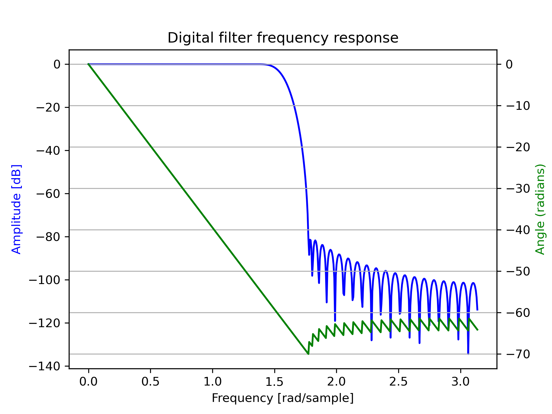
Compute the frequency response of a digital filter.
>>> from scipy import signal
... b = signal.firwin(80, 0.5, window=('kaiser', 8))
... w, h = signal.freqz(b)
>>> import matplotlib.pyplot as plt
... fig, ax1 = plt.subplots()
... ax1.set_title('Digital filter frequency response')
>>> ax1.plot(w, 20 * np.log10(abs(h)), 'b')
... ax1.set_ylabel('Amplitude [dB]', color='b')
... ax1.set_xlabel('Frequency [rad/sample]')
>>> ax2 = ax1.twinx()
... angles = np.unwrap(np.angle(h))
... ax2.plot(w, angles, 'g')
... ax2.set_ylabel('Angle (radians)', color='g')
... ax2.grid()
... ax2.axis('tight')
... plt.show()
Broadcasting Examples
Suppose we have two FIR filters whose coefficients are stored in the rows of an array with shape (2, 25). For this demonstration, we'll use random data:
>>> rng = np.random.default_rng()
... b = rng.random((2, 25))
To compute the frequency response for these two filters with one call to freqz
, we must pass in b.T
, because freqz
expects the first axis to hold the coefficients. We must then extend the shape with a trivial dimension of length 1 to allow broadcasting with the array of frequencies. That is, we pass in b.T[..., np.newaxis]
, which has shape (25, 2, 1):
>>> w, h = signal.freqz(b.T[..., np.newaxis], worN=1024)
... w.shape
(1024,)
>>> h.shape
(2, 1024)
a = [ 1 1 ]
[ -0.25, -0.5 ]
>>> b = np.array([0.5, 0.5])
... a = np.array([[1, 1], [-0.25, -0.5]])
Only a is more than 1-D. To make it compatible for broadcasting with the frequencies, we extend it with a trivial dimension in the call to freqz
:
>>> w, h = signal.freqz(b, a[..., np.newaxis], worN=1024)
... w.shape
(1024,)
>>> h.shape
(2, 1024)
See :
The following pages refer to to this document either explicitly or contain code examples using this.
scipy.signal._filter_design.sosfreqz
scipy.signal._filter_design.gammatone
scipy.signal._filter_design.freqs
scipy.signal._fir_filter_design.minimum_phase
scipy.signal._fir_filter_design.kaiserord
scipy.signal._filter_design.iirnotch
scipy.signal._filter_design.freqz
scipy.signal._filter_design.iirpeak
scipy.signal._fir_filter_design.remez
scipy.signal._filter_design.group_delay
scipy.signal._fir_filter_design.firls
scipy.signal._filter_design.freqz_zpk
scipy.signal._filter_design.freqs_zpk
scipy.signal._filter_design.iircomb
scipy.signal._filter_design.bilinear
scipy.signal._filter_design.iirdesign
scipy.signal._filter_design.cheb1ord
scipy.signal.windows._windows.dpss
scipy.signal._filter_design.cheb2ord
Hover to see nodes names; edges to Self not shown, Caped at 50 nodes.
Using a canvas is more power efficient and can get hundred of nodes ; but does not allow hyperlinks; , arrows or text (beyond on hover)
SVG is more flexible but power hungry; and does not scale well to 50 + nodes.
All aboves nodes referred to, (or are referred from) current nodes; Edges from Self to other have been omitted (or all nodes would be connected to the central node "self" which is not useful). Nodes are colored by the library they belong to, and scaled with the number of references pointing them