dpss(M, NW, Kmax=None, sym=True, norm=None, return_ratios=False)
DPSS (or Slepian sequences) are often used in multitaper power spectral density estimation (see ). The first window in the sequence can be used to maximize the energy concentration in the main lobe, and is also called the Slepian window.
This computation uses the tridiagonal eigenvector formulation given in .
The default normalization for Kmax=None
, i.e. window-generation mode, simply using the l-infinity norm would create a window with two unity values, which creates slight normalization differences between even and odd orders. The approximate correction of M**2/float(M**2+NW)
for even sample numbers is used to counteract this effect (see Examples below).
For very long signals (e.g., 1e6 elements), it can be useful to compute windows orders of magnitude shorter and use interpolation (e.g., scipy.interpolate.interp1d
) to obtain tapers of length M, but this in general will not preserve orthogonality between the tapers.
Window length.
Standardized half bandwidth corresponding to 2*NW = BW/f0 = BW*M*dt
where dt
is taken as 1.
Number of DPSS windows to return (orders 0
through Kmax-1
). If None (default), return only a single window of shape (M,)
instead of an array of windows of shape (Kmax, M)
.
When True (default), generates a symmetric window, for use in filter design. When False, generates a periodic window, for use in spectral analysis.
If 'approximate' or 'subsample', then the windows are normalized by the maximum, and a correction scale-factor for even-length windows is applied either using M**2/(M**2+NW)
("approximate") or a FFT-based subsample shift ("subsample"), see Notes for details. If None, then "approximate" is used when Kmax=None
and 2 otherwise (which uses the l2 norm).
If True, also return the concentration ratios in addition to the windows.
The DPSS windows. Will be 1D if :None:None:`Kmax` is None.
The concentration ratios for the windows. Only returned if :None:None:`return_ratios` evaluates to True. Will be 0D if :None:None:`Kmax` is None.
Compute the Discrete Prolate Spheroidal Sequences (DPSS).
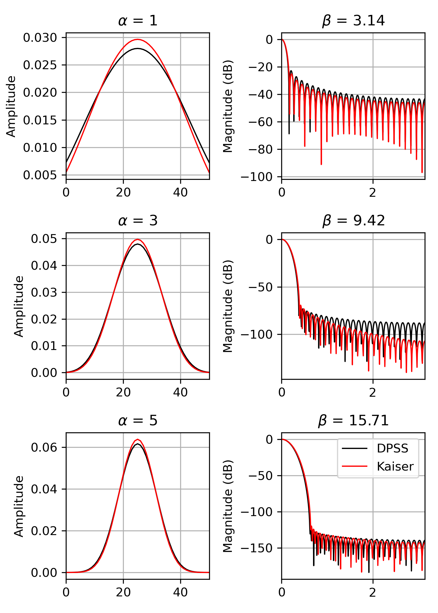
We can compare the window to kaiser
, which was invented as an alternative that was easier to calculate (example adapted from here):
>>> import numpy as np
... import matplotlib.pyplot as plt
... from scipy.signal import windows, freqz
... M = 51
... fig, axes = plt.subplots(3, 2, figsize=(5, 7))
... for ai, alpha in enumerate((1, 3, 5)):
...     win_dpss = windows.dpss(M, alpha)
...     beta = alpha*np.pi
...     win_kaiser = windows.kaiser(M, beta)
...     for win, c in ((win_dpss, 'k'), (win_kaiser, 'r')):
...         win /= win.sum()
...         axes[ai, 0].plot(win, color=c, lw=1.)
...         axes[ai, 0].set(xlim=[0, M-1], title=r'$\alpha$ = %s' % alpha,
...                         ylabel='Amplitude')
...         w, h = freqz(win)
...         axes[ai, 1].plot(w, 20 * np.log10(np.abs(h)), color=c, lw=1.)
...         axes[ai, 1].set(xlim=[0, np.pi],
...                         title=r'$\beta$ = %0.2f' % beta,
...                         ylabel='Magnitude (dB)')
... for ax in axes.ravel():
...     ax.grid(True)
... axes[2, 1].legend(['DPSS', 'Kaiser'])
... fig.tight_layout()
... plt.show()
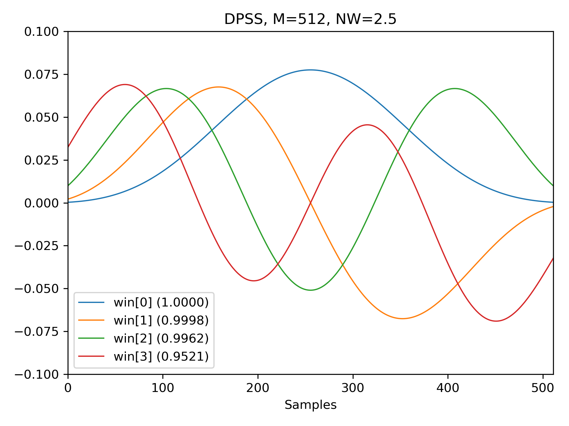
And here are examples of the first four windows, along with their concentration ratios:
>>> M = 512
... NW = 2.5
... win, eigvals = windows.dpss(M, NW, 4, return_ratios=True)
... fig, ax = plt.subplots(1)
... ax.plot(win.T, linewidth=1.)
... ax.set(xlim=[0, M-1], ylim=[-0.1, 0.1], xlabel='Samples',
...        title='DPSS, M=%d, NW=%0.1f' % (M, NW))
... ax.legend(['win[%d] (%0.4f)' % (ii, ratio)
...            for ii, ratio in enumerate(eigvals)])
... fig.tight_layout()
... plt.show()
Using a standard $l_{\infty}$
norm would produce two unity values for even M, but only one unity value for odd M. This produces uneven window power that can be counteracted by the approximate correction M**2/float(M**2+NW)
, which can be selected by using norm='approximate'
(which is the same as norm=None
when Kmax=None
, as is the case here). Alternatively, the slower norm='subsample'
can be used, which uses subsample shifting in the frequency domain (FFT) to compute the correction:
>>> Ms = np.arange(1, 41)See :
... factors = (50, 20, 10, 5, 2.0001)
... energy = np.empty((3, len(Ms), len(factors)))
... for mi, M in enumerate(Ms):
... for fi, factor in enumerate(factors):
... NW = M / float(factor)
... # Corrected using empirical approximation (default)
... win = windows.dpss(M, NW)
... energy[0, mi, fi] = np.sum(win ** 2) / np.sqrt(M)
... # Corrected using subsample shifting
... win = windows.dpss(M, NW, norm='subsample')
... energy[1, mi, fi] = np.sum(win ** 2) / np.sqrt(M)
... # Uncorrected (using l-infinity norm)
... win /= win.max()
... energy[2, mi, fi] = np.sum(win ** 2) / np.sqrt(M)
... fig, ax = plt.subplots(1)
... hs = ax.plot(Ms, energy[2], '-o', markersize=4,
... markeredgecolor='none')
... leg = [hs[-1]]
... for hi, hh in enumerate(hs):
... h1 = ax.plot(Ms, energy[0, :, hi], '-o', markersize=4,
... color=hh.get_color(), markeredgecolor='none',
... alpha=0.66)
... h2 = ax.plot(Ms, energy[1, :, hi], '-o', markersize=4,
... color=hh.get_color(), markeredgecolor='none',
... alpha=0.33)
... if hi == len(hs) - 1:
... leg.insert(0, h1[0])
... leg.insert(0, h2[0])
... ax.set(xlabel='M (samples)', ylabel=r'Power / $\sqrt{M}$')
... ax.legend(leg, ['Uncorrected', r'Corrected: $\frac{M^2}{M^2+NW}$',
... 'Corrected (subsample)'])
... fig.tight_layout()
The following pages refer to to this document either explicitly or contain code examples using this.
scipy.signal.windows._windows.dpss
scipy.signal.windows._windows.get_window
papyri
Hover to see nodes names; edges to Self not shown, Caped at 50 nodes.
Using a canvas is more power efficient and can get hundred of nodes ; but does not allow hyperlinks; , arrows or text (beyond on hover)
SVG is more flexible but power hungry; and does not scale well to 50 + nodes.
All aboves nodes referred to, (or are referred from) current nodes; Edges from Self to other have been omitted (or all nodes would be connected to the central node "self" which is not useful). Nodes are colored by the library they belong to, and scaled with the number of references pointing them