general_cosine(M, a, sym=True)
Number of points in the output window
Sequence of weighting coefficients. This uses the convention of being centered on the origin, so these will typically all be positive numbers, not alternating sign.
When True (default), generates a symmetric window, for use in filter design. When False, generates a periodic window, for use in spectral analysis.
Generic weighted sum of cosine terms window
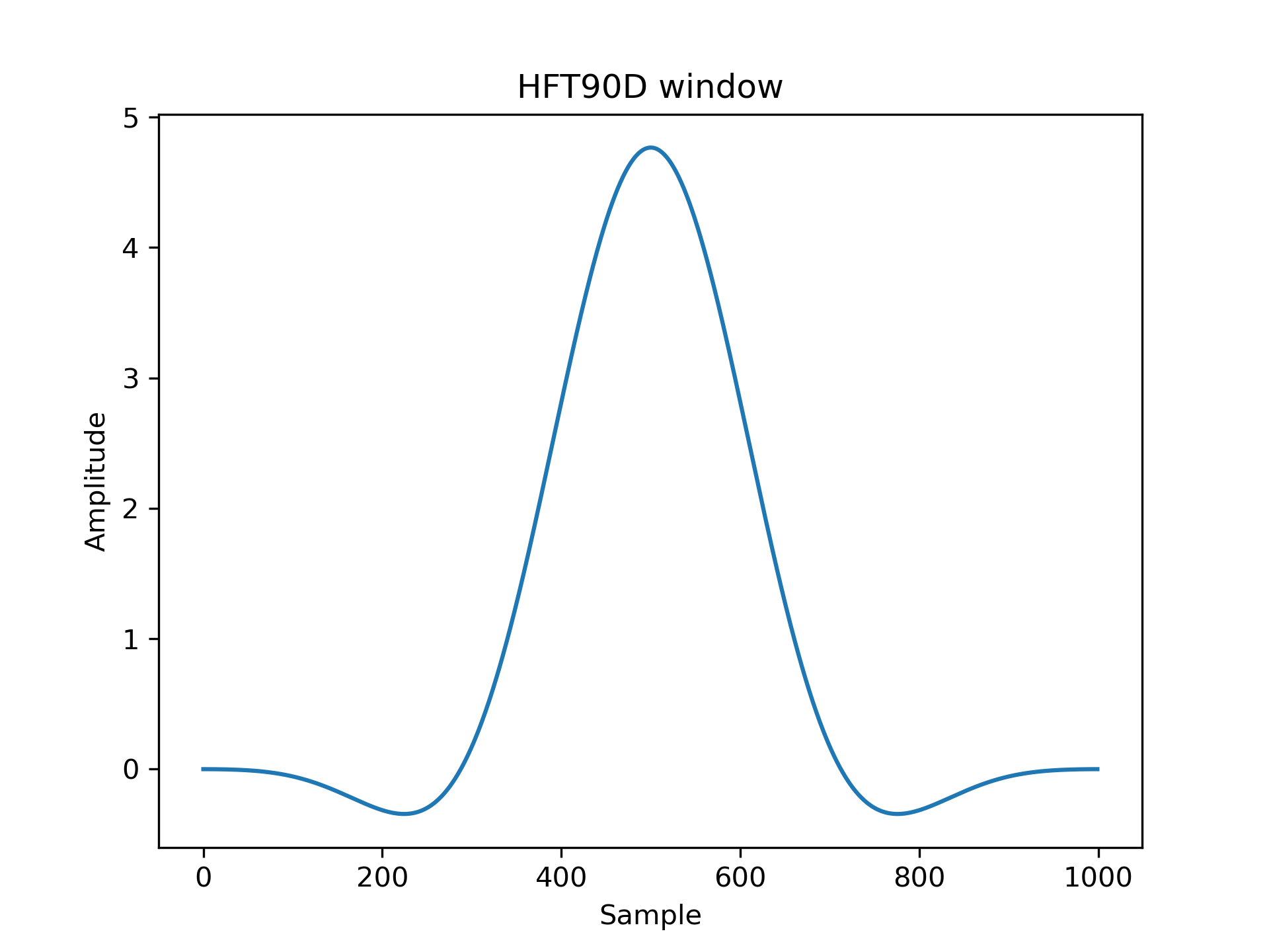
Heinzel describes a flat-top window named "HFT90D" with formula:
$$w_j = 1 - 1.942604 \cos(z) + 1.340318 \cos(2z)- 0.440811 \cos(3z) + 0.043097 \cos(4z)$$where
$$z = \frac{2 \pi j}{N}, j = 0...N - 1$$Since this uses the convention of starting at the origin, to reproduce the window, we need to convert every other coefficient to a positive number:
>>> HFT90D = [1, 1.942604, 1.340318, 0.440811, 0.043097]
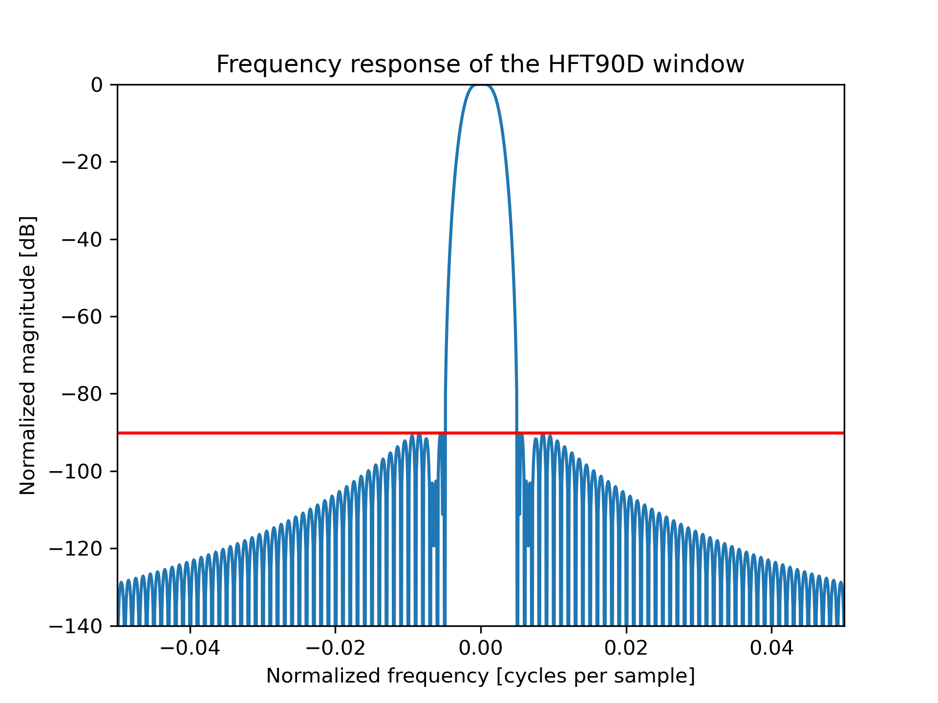
The paper states that the highest sidelobe is at -90.2 dB. Reproduce Figure 42 by plotting the window and its frequency response, and confirm the sidelobe level in red:
>>> from scipy.signal.windows import general_cosine
... from scipy.fft import fft, fftshift
... import matplotlib.pyplot as plt
>>> window = general_cosine(1000, HFT90D, sym=False)
... plt.plot(window)
... plt.title("HFT90D window")
... plt.ylabel("Amplitude")
... plt.xlabel("Sample")
>>> plt.figure()
... A = fft(window, 10000) / (len(window)/2.0)
... freq = np.linspace(-0.5, 0.5, len(A))
... response = np.abs(fftshift(A / abs(A).max()))
... response = 20 * np.log10(np.maximum(response, 1e-10))
... plt.plot(freq, response)
... plt.axis([-50/1000, 50/1000, -140, 0])
... plt.title("Frequency response of the HFT90D window")
... plt.ylabel("Normalized magnitude [dB]")
... plt.xlabel("Normalized frequency [cycles per sample]")
... plt.axhline(-90.2, color='red')
... plt.show()
The following pages refer to to this document either explicitly or contain code examples using this.
scipy.signal.windows._windows.get_window
scipy.signal.windows._windows.general_cosine
Hover to see nodes names; edges to Self not shown, Caped at 50 nodes.
Using a canvas is more power efficient and can get hundred of nodes ; but does not allow hyperlinks; , arrows or text (beyond on hover)
SVG is more flexible but power hungry; and does not scale well to 50 + nodes.
All aboves nodes referred to, (or are referred from) current nodes; Edges from Self to other have been omitted (or all nodes would be connected to the central node "self" which is not useful). Nodes are colored by the library they belong to, and scaled with the number of references pointing them