kaiserord(ripple, width)
The parameters returned by this function are generally used to create a finite impulse response filter using the window method, with either firwin
or firwin2
.
There are several ways to obtain the Kaiser window:
signal.windows.kaiser(numtaps, beta, sym=True)
signal.get_window(beta, numtaps)
signal.get_window(('kaiser', beta), numtaps)
The empirical equations discovered by Kaiser are used.
Upper bound for the deviation (in dB) of the magnitude of the filter's frequency response from that of the desired filter (not including frequencies in any transition intervals). That is, if w is the frequency expressed as a fraction of the Nyquist frequency, A(w) is the actual frequency response of the filter and D(w) is the desired frequency response, the design requirement is that:
abs(A(w) - D(w))) < 10**(-ripple/20)
for 0 <= w <= 1 and w not in a transition interval.
Width of transition region, normalized so that 1 corresponds to pi radians / sample. That is, the frequency is expressed as a fraction of the Nyquist frequency.
The length of the Kaiser window.
The beta parameter for the Kaiser window.
Determine the filter window parameters for the Kaiser window method.
We will use the Kaiser window method to design a lowpass FIR filter for a signal that is sampled at 1000 Hz.
We want at least 65 dB rejection in the stop band, and in the pass band the gain should vary no more than 0.5%.
We want a cutoff frequency of 175 Hz, with a transition between the pass band and the stop band of 24 Hz. That is, in the band [0, 163], the gain varies no more than 0.5%, and in the band [187, 500], the signal is attenuated by at least 65 dB.
>>> from scipy.signal import kaiserord, firwin, freqz
... import matplotlib.pyplot as plt
... fs = 1000.0
... cutoff = 175
... width = 24
The Kaiser method accepts just a single parameter to control the pass band ripple and the stop band rejection, so we use the more restrictive of the two. In this case, the pass band ripple is 0.005, or 46.02 dB, so we will use 65 dB as the design parameter.
Use kaiserord
to determine the length of the filter and the parameter for the Kaiser window.
>>> numtaps, beta = kaiserord(65, width/(0.5*fs))
... numtaps
167
>>> beta
6.20426
Use firwin
to create the FIR filter.
>>> taps = firwin(numtaps, cutoff, window=('kaiser', beta),
...               scale=False, nyq=0.5*fs)
Compute the frequency response of the filter. w
is the array of frequencies, and h
is the corresponding complex array of frequency responses.
>>> w, h = freqz(taps, worN=8000)
... w *= 0.5*fs/np.pi  # Convert w to Hz.
Compute the deviation of the magnitude of the filter's response from that of the ideal lowpass filter. Values in the transition region are set to nan
, so they won't appear in the plot.
>>> ideal = w < cutoff  # The "ideal" frequency response.
... deviation = np.abs(np.abs(h) - ideal)
... deviation[(w > cutoff - 0.5*width) & (w < cutoff + 0.5*width)] = np.nan
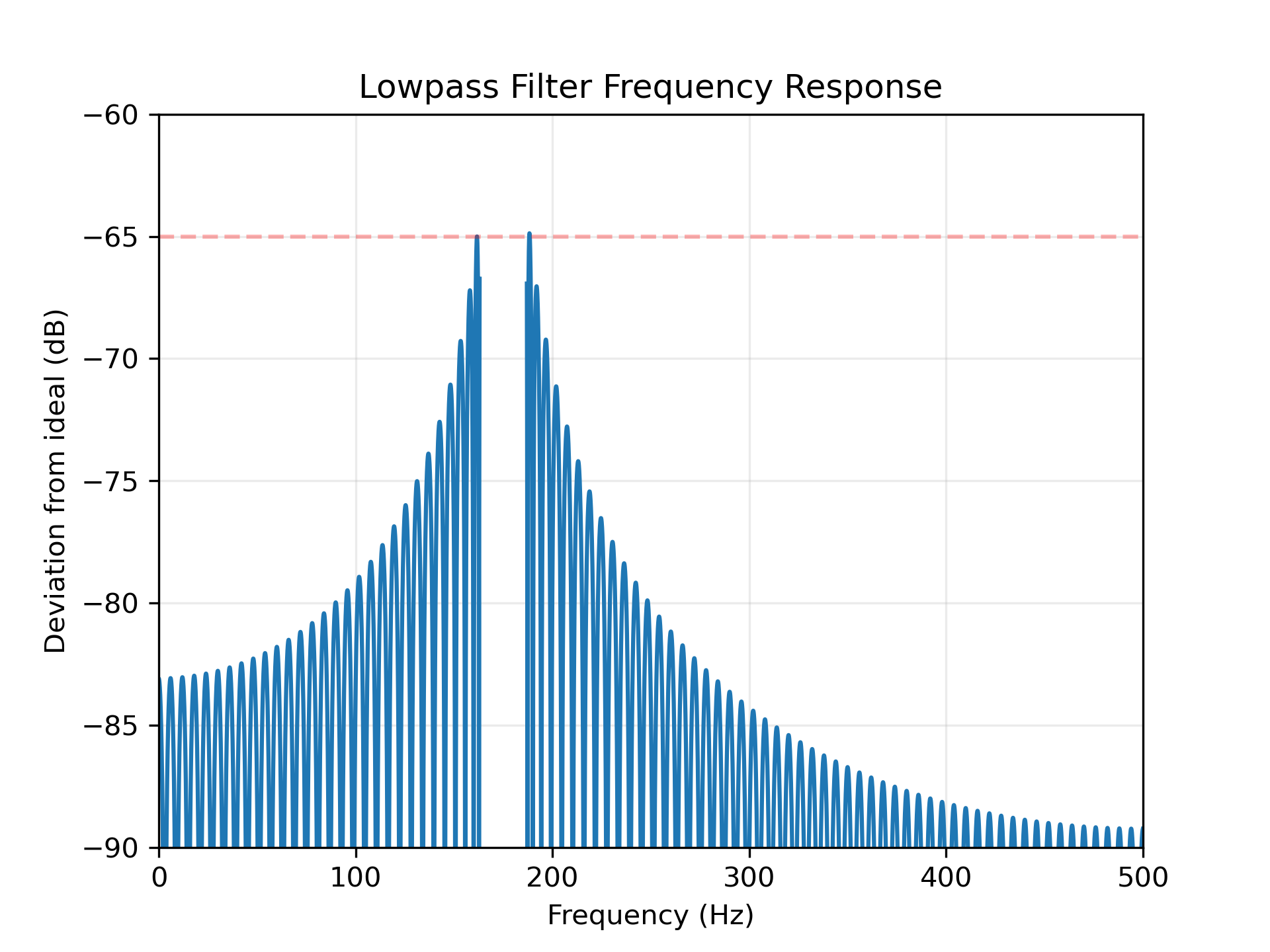
Plot the deviation. A close look at the left end of the stop band shows that the requirement for 65 dB attenuation is violated in the first lobe by about 0.125 dB. This is not unusual for the Kaiser window method.
>>> plt.plot(w, 20*np.log10(np.abs(deviation)))
... plt.xlim(0, 0.5*fs)
... plt.ylim(-90, -60)
... plt.grid(alpha=0.25)
... plt.axhline(-65, color='r', ls='--', alpha=0.3)
... plt.xlabel('Frequency (Hz)')
... plt.ylabel('Deviation from ideal (dB)')
... plt.title('Lowpass Filter Frequency Response')
... plt.show()
The following pages refer to to this document either explicitly or contain code examples using this.
scipy.signal._fir_filter_design.kaiserord
scipy.signal._fir_filter_design.kaiser_atten
Hover to see nodes names; edges to Self not shown, Caped at 50 nodes.
Using a canvas is more power efficient and can get hundred of nodes ; but does not allow hyperlinks; , arrows or text (beyond on hover)
SVG is more flexible but power hungry; and does not scale well to 50 + nodes.
All aboves nodes referred to, (or are referred from) current nodes; Edges from Self to other have been omitted (or all nodes would be connected to the central node "self" which is not useful). Nodes are colored by the library they belong to, and scaled with the number of references pointing them