Document

scipy 1.8.0 Pypi GitHub Homepage

sosfilt(sos, x, axis=-1, zi=None)

Filter a data sequence, x, using a digital IIR filter defined by :None:None:`sos`.

Notes

The filter function is implemented as a series of second-order filters with direct-form II transposed structure. It is designed to minimize numerical precision errors for high-order filters.

versionadded

Parameters

sos : array_like: Array of second-order filter coefficients, must have shape (n_sections, 6) . Each row corresponds to a second-order section, with the first three columns providing the numerator coefficients and the last three providing the denominator coefficients.
x : array_like: An N-dimensional input array.
axis : int, optional: The axis of the input data array along which to apply the linear filter. The filter is applied to each subarray along this axis. Default is -1.
zi : array_like, optional: Initial conditions for the cascaded filter delays. It is a (at least 2D) vector of shape (n_sections, ..., 2, ...) , where ..., 2, ... denotes the shape of x, but with x.shape[axis] replaced by 2. If :None:None:`zi` is None or is not given then initial rest (i.e. all zeros) is assumed. Note that these initial conditions are not the same as the initial conditions given by lfiltic or lfilter_zi .

Returns

y : ndarray: The output of the digital filter.
zf : ndarray, optional: If :None:None:`zi` is None, this is not returned, otherwise, :None:None:`zf` holds the final filter delay values.

Filter data along one dimension using cascaded second-order sections.

Examples

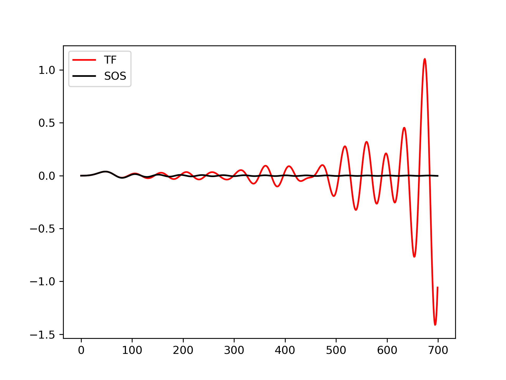
Plot a 13th-order filter's impulse response using both lfilter and sosfilt , showing the instability that results from trying to do a 13th-order filter in a single stage (the numerical error pushes some poles outside of the unit circle):

>>> import matplotlib.pyplot as plt
... from scipy import signal
... b, a = signal.ellip(13, 0.009, 80, 0.05, output='ba')
... sos = signal.ellip(13, 0.009, 80, 0.05, output='sos')
... x = signal.unit_impulse(700)
... y_tf = signal.lfilter(b, a, x)
... y_sos = signal.sosfilt(sos, x)
... plt.plot(y_tf, 'r', label='TF')
... plt.plot(y_sos, 'k', label='SOS')
... plt.legend(loc='best')
... plt.show()

See :

Back References

The following pages refer to to this document either explicitly or contain code examples using this.

scipy.signal._filter_design.butter scipy.signal._signaltools.sosfiltfilt scipy.signal._filter_design.ellip scipy.signal._filter_design.cheby1 scipy.signal._signaltools.lfilter scipy.signal._filter_design.zpk2sos scipy.signal._signaltools.filtfilt scipy.signal._filter_design.sos2zpk scipy.signal._filter_design.cheby2 scipy.signal._filter_design.sos2tf scipy.signal._filter_design.sosfreqz scipy.signal._signaltools.sosfilt_zi scipy.signal._signaltools.sosfilt scipy.signal._filter_design.tf2sos

Local connectivity graph

Hover to see nodes names; edges to Self not shown, Caped at 50 nodes.

Using a canvas is more power efficient and can get hundred of nodes ; but does not allow hyperlinks; , arrows or text (beyond on hover)

SVG is more flexible but power hungry; and does not scale well to 50 + nodes.

All aboves nodes referred to, (or are referred from) current nodes; Edges from Self to other have been omitted (or all nodes would be connected to the central node "self" which is not useful). Nodes are colored by the library they belong to, and scaled with the number of references pointing them