filtfilt(b, a, x, axis=-1, padtype='odd', padlen=None, method='pad', irlen=None)
This function applies a linear digital filter twice, once forward and once backwards. The combined filter has zero phase and a filter order twice that of the original.
The function provides options for handling the edges of the signal.
The function sosfiltfilt
(and filter design using output='sos'
) should be preferred over filtfilt
for most filtering tasks, as second-order sections have fewer numerical problems.
When method
is "pad", the function pads the data along the given axis in one of three ways: odd, even or constant. The odd and even extensions have the corresponding symmetry about the end point of the data. The constant extension extends the data with the values at the end points. On both the forward and backward passes, the initial condition of the filter is found by using lfilter_zi
and scaling it by the end point of the extended data.
When method
is "gust", Gustafsson's method is used. Initial conditions are chosen for the forward and backward passes so that the forward-backward filter gives the same result as the backward-forward filter.
The option to use Gustaffson's method was added in scipy version 0.16.0.
The numerator coefficient vector of the filter.
The denominator coefficient vector of the filter. If a[0]
is not 1, then both a and b are normalized by a[0]
.
The array of data to be filtered.
The axis of x to which the filter is applied. Default is -1.
Must be 'odd', 'even', 'constant', or None. This determines the type of extension to use for the padded signal to which the filter is applied. If :None:None:`padtype` is None, no padding is used. The default is 'odd'.
The number of elements by which to extend x at both ends of :None:None:`axis` before applying the filter. This value must be less than x.shape[axis] - 1
. padlen=0
implies no padding. The default value is 3 * max(len(a), len(b))
.
Determines the method for handling the edges of the signal, either "pad" or "gust". When method
is "pad", the signal is padded; the type of padding is determined by :None:None:`padtype` and :None:None:`padlen`, and :None:None:`irlen` is ignored. When method
is "gust", Gustafsson's method is used, and :None:None:`padtype` and :None:None:`padlen` are ignored.
When method
is "gust", :None:None:`irlen` specifies the length of the impulse response of the filter. If :None:None:`irlen` is None, no part of the impulse response is ignored. For a long signal, specifying :None:None:`irlen` can significantly improve the performance of the filter.
Apply a digital filter forward and backward to a signal.
The examples will use several functions from scipy.signal
.
>>> from scipy import signal
... import matplotlib.pyplot as plt
First we create a one second signal that is the sum of two pure sine waves, with frequencies 5 Hz and 250 Hz, sampled at 2000 Hz.
>>> t = np.linspace(0, 1.0, 2001)
... xlow = np.sin(2 * np.pi * 5 * t)
... xhigh = np.sin(2 * np.pi * 250 * t)
... x = xlow + xhigh
Now create a lowpass Butterworth filter with a cutoff of 0.125 times the Nyquist frequency, or 125 Hz, and apply it to x
with filtfilt
. The result should be approximately xlow
, with no phase shift.
>>> b, a = signal.butter(8, 0.125)
... y = signal.filtfilt(b, a, x, padlen=150)
... np.abs(y - xlow).max()
9.1086182074789912e-06
We get a fairly clean result for this artificial example because the odd extension is exact, and with the moderately long padding, the filter's transients have dissipated by the time the actual data is reached. In general, transient effects at the edges are unavoidable.
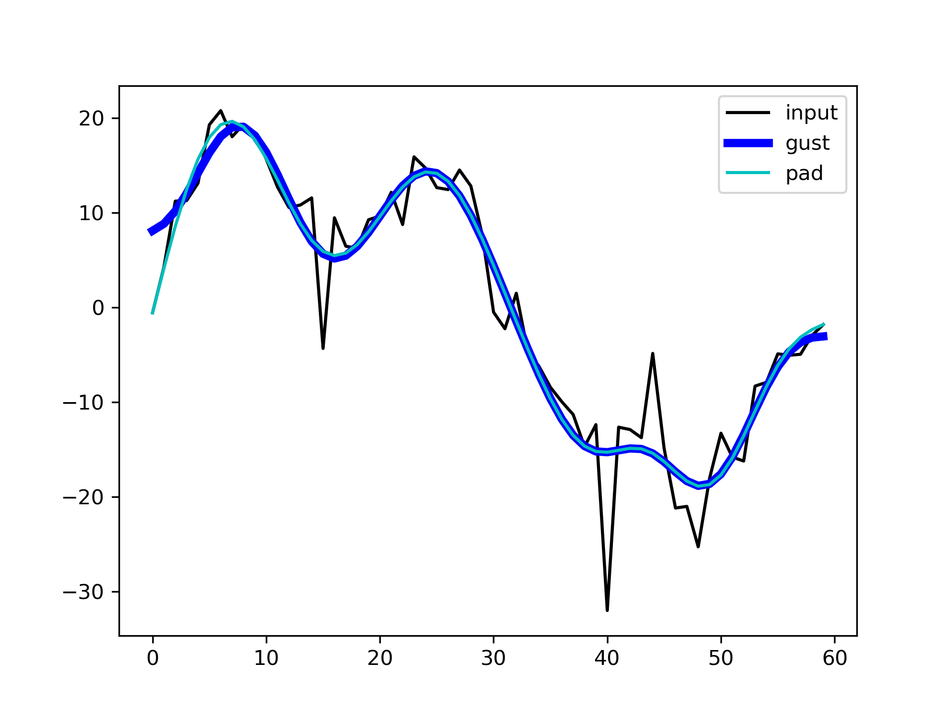
The following example demonstrates the option method="gust"
.
First, create a filter.
>>> b, a = signal.ellip(4, 0.01, 120, 0.125) # Filter to be applied.
:None:None:`sig` is a random input signal to be filtered.
>>> rng = np.random.default_rng()
... n = 60
... sig = rng.standard_normal(n)**3 + 3*rng.standard_normal(n).cumsum()
Apply filtfilt
to :None:None:`sig`, once using the Gustafsson method, and once using padding, and plot the results for comparison.
>>> fgust = signal.filtfilt(b, a, sig, method="gust")
... fpad = signal.filtfilt(b, a, sig, padlen=50)
... plt.plot(sig, 'k-', label='input')
... plt.plot(fgust, 'b-', linewidth=4, label='gust')
... plt.plot(fpad, 'c-', linewidth=1.5, label='pad')
... plt.legend(loc='best')
... plt.show()
The :None:None:`irlen` argument can be used to improve the performance of Gustafsson's method.
Estimate the impulse response length of the filter.
>>> z, p, k = signal.tf2zpk(b, a)
... eps = 1e-9
... r = np.max(np.abs(p))
... approx_impulse_len = int(np.ceil(np.log(eps) / np.log(r)))
... approx_impulse_len
137
Apply the filter to a longer signal, with and without the :None:None:`irlen` argument. The difference between y1
and y2
is small. For long signals, using :None:None:`irlen` gives a significant performance improvement.
>>> x = rng.standard_normal(5000)See :
... y1 = signal.filtfilt(b, a, x, method='gust')
... y2 = signal.filtfilt(b, a, x, method='gust', irlen=approx_impulse_len)
... print(np.max(np.abs(y1 - y2))) 1.80056858312e-10
The following pages refer to to this document either explicitly or contain code examples using this.
scipy.signal._signaltools.sosfiltfilt
scipy.signal._signaltools.lfilter
scipy.signal._signaltools.filtfilt
scipy.signal._signaltools.decimate
scipy.signal._signaltools.lfilter_zi
Hover to see nodes names; edges to Self not shown, Caped at 50 nodes.
Using a canvas is more power efficient and can get hundred of nodes ; but does not allow hyperlinks; , arrows or text (beyond on hover)
SVG is more flexible but power hungry; and does not scale well to 50 + nodes.
All aboves nodes referred to, (or are referred from) current nodes; Edges from Self to other have been omitted (or all nodes would be connected to the central node "self" which is not useful). Nodes are colored by the library they belong to, and scaled with the number of references pointing them