resample_poly(x, up, down, axis=0, window=('kaiser', 5.0), padtype='constant', cval=None)
The signal x is upsampled by the factor :None:None:`up`, a zero-phase low-pass FIR filter is applied, and then it is downsampled by the factor down
. The resulting sample rate is up / down
times the original sample rate. By default, values beyond the boundary of the signal are assumed to be zero during the filtering step.
This polyphase method will likely be faster than the Fourier method in scipy.signal.resample
when the number of samples is large and prime, or when the number of samples is large and :None:None:`up` and down
share a large greatest common denominator. The length of the FIR filter used will depend on max(up, down) // gcd(up, down)
, and the number of operations during polyphase filtering will depend on the filter length and down
(see scipy.signal.upfirdn
for details).
The argument :None:None:`window` specifies the FIR low-pass filter design.
If :None:None:`window` is an array_like it is assumed to be the FIR filter coefficients. Note that the FIR filter is applied after the upsampling step, so it should be designed to operate on a signal at a sampling frequency higher than the original by a factor of :None:None:`up//gcd(up, down)`. This function's output will be centered with respect to this array, so it is best to pass a symmetric filter with an odd number of samples if, as is usually the case, a zero-phase filter is desired.
For any other type of :None:None:`window`, the functions scipy.signal.get_window
and scipy.signal.firwin
are called to generate the appropriate filter coefficients.
The first sample of the returned vector is the same as the first sample of the input vector. The spacing between samples is changed from dx
to dx * down / float(up)
.
The data to be resampled.
The upsampling factor.
The downsampling factor.
The axis of x that is resampled. Default is 0.
Desired window to use to design the low-pass filter, or the FIR filter coefficients to employ. See below for details.
constant
, :None:None:`line`, mean
, median
, :None:None:`maximum`, :None:None:`minimum` or any of the other signal extension modes supported by scipy.signal.upfirdn
. Changes assumptions on values beyond the boundary. If constant
, assumed to be :None:None:`cval` (default zero). If :None:None:`line` assumed to continue a linear trend defined by the first and last points. mean
, median
, :None:None:`maximum` and :None:None:`minimum` work as in :None:None:`np.pad` and assume that the values beyond the boundary are the mean, median, maximum or minimum respectively of the array along the axis.
Value to use if :None:None:`padtype='constant'`. Default is zero.
The resampled array.
Resample x along the given axis using polyphase filtering.
decimate
Downsample the signal after applying an FIR or IIR filter.
resample
Resample up or down using the FFT method.
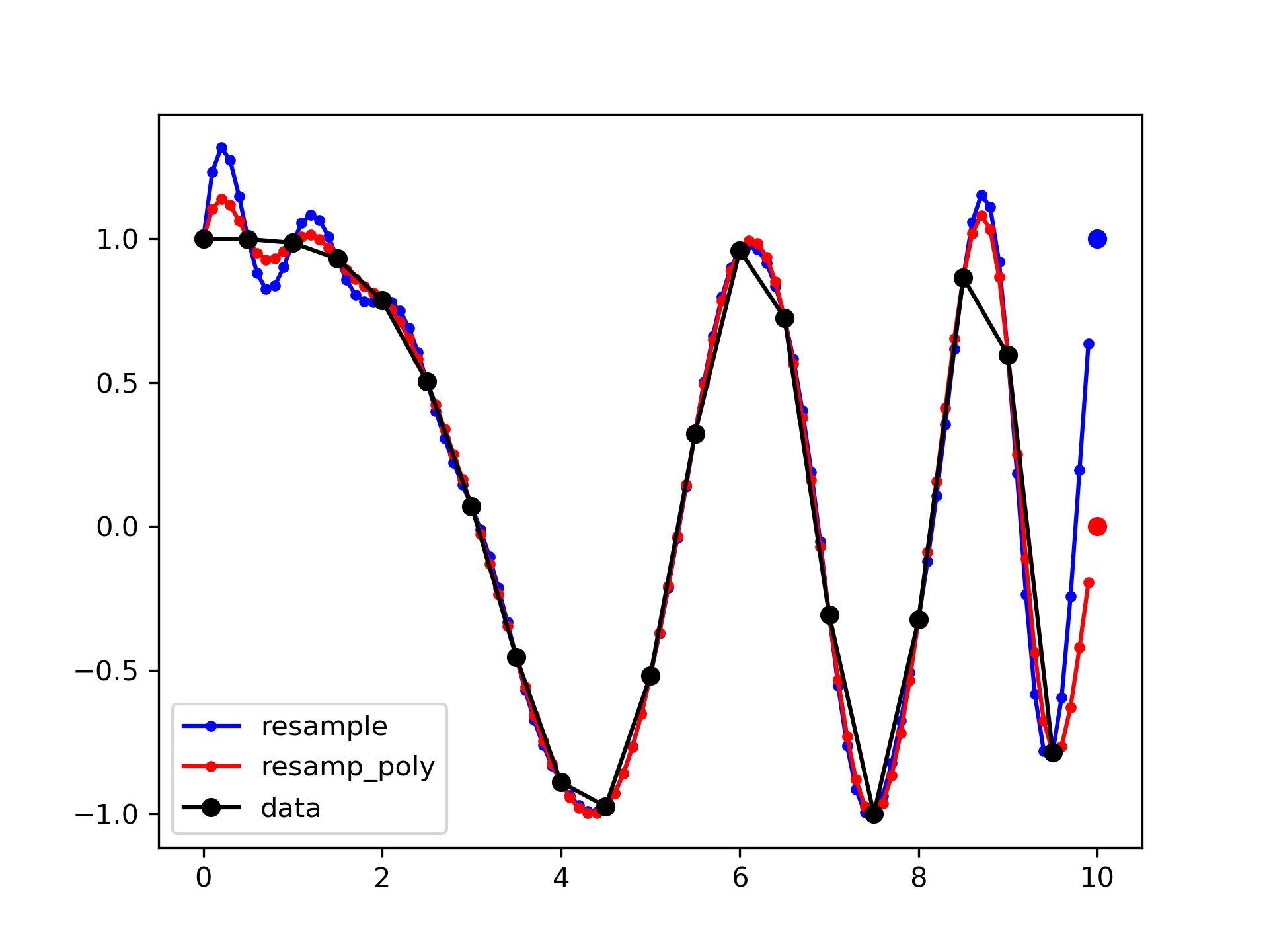
By default, the end of the resampled data rises to meet the first sample of the next cycle for the FFT method, and gets closer to zero for the polyphase method:
>>> from scipy import signal
>>> x = np.linspace(0, 10, 20, endpoint=False)
... y = np.cos(-x**2/6.0)
... f_fft = signal.resample(y, 100)
... f_poly = signal.resample_poly(y, 100, 20)
... xnew = np.linspace(0, 10, 100, endpoint=False)
>>> import matplotlib.pyplot as plt
... plt.plot(xnew, f_fft, 'b.-', xnew, f_poly, 'r.-')
... plt.plot(x, y, 'ko-')
... plt.plot(10, y[0], 'bo', 10, 0., 'ro')  # boundaries
... plt.legend(['resample', 'resamp_poly', 'data'], loc='best')
... plt.show()
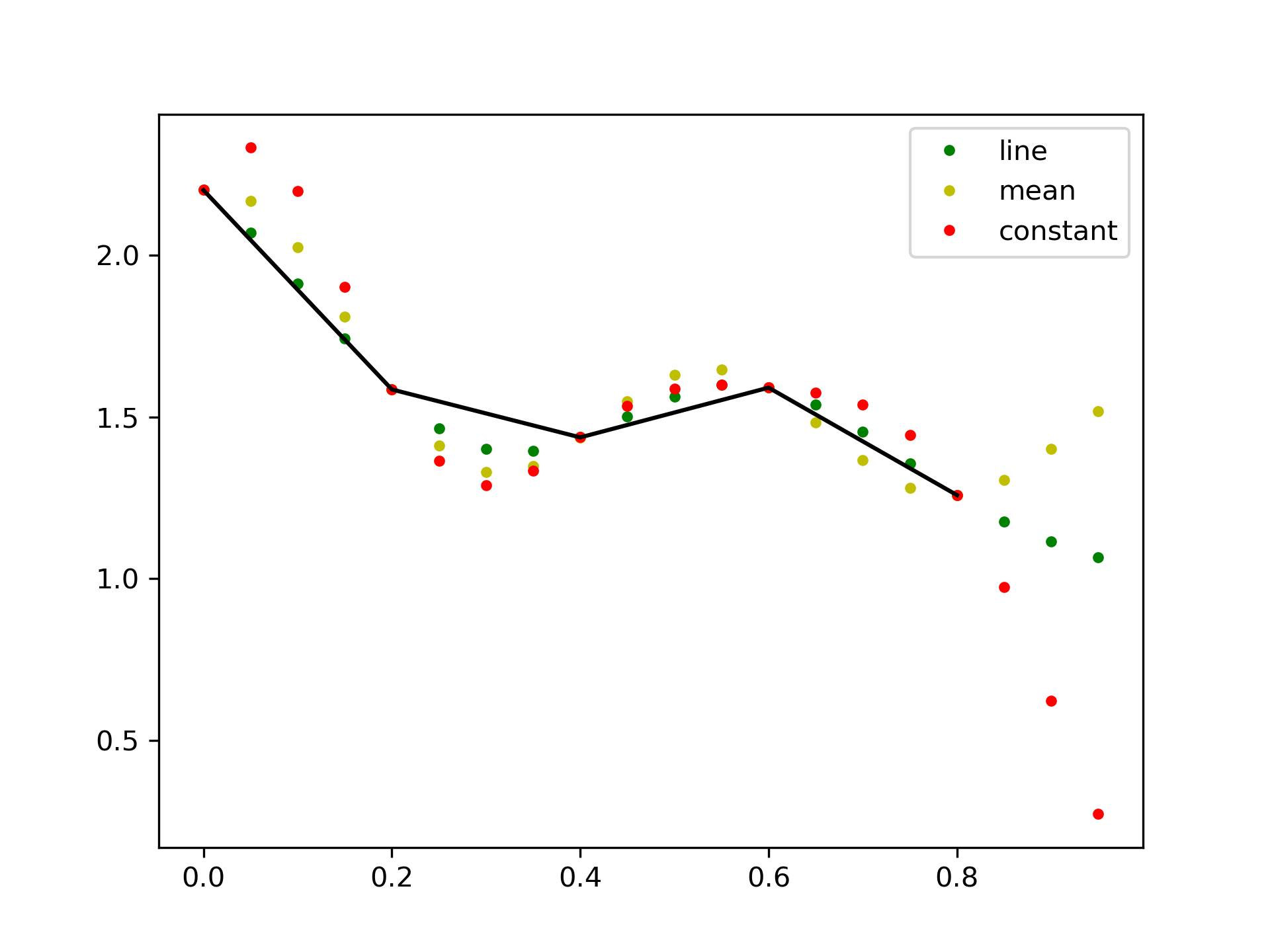
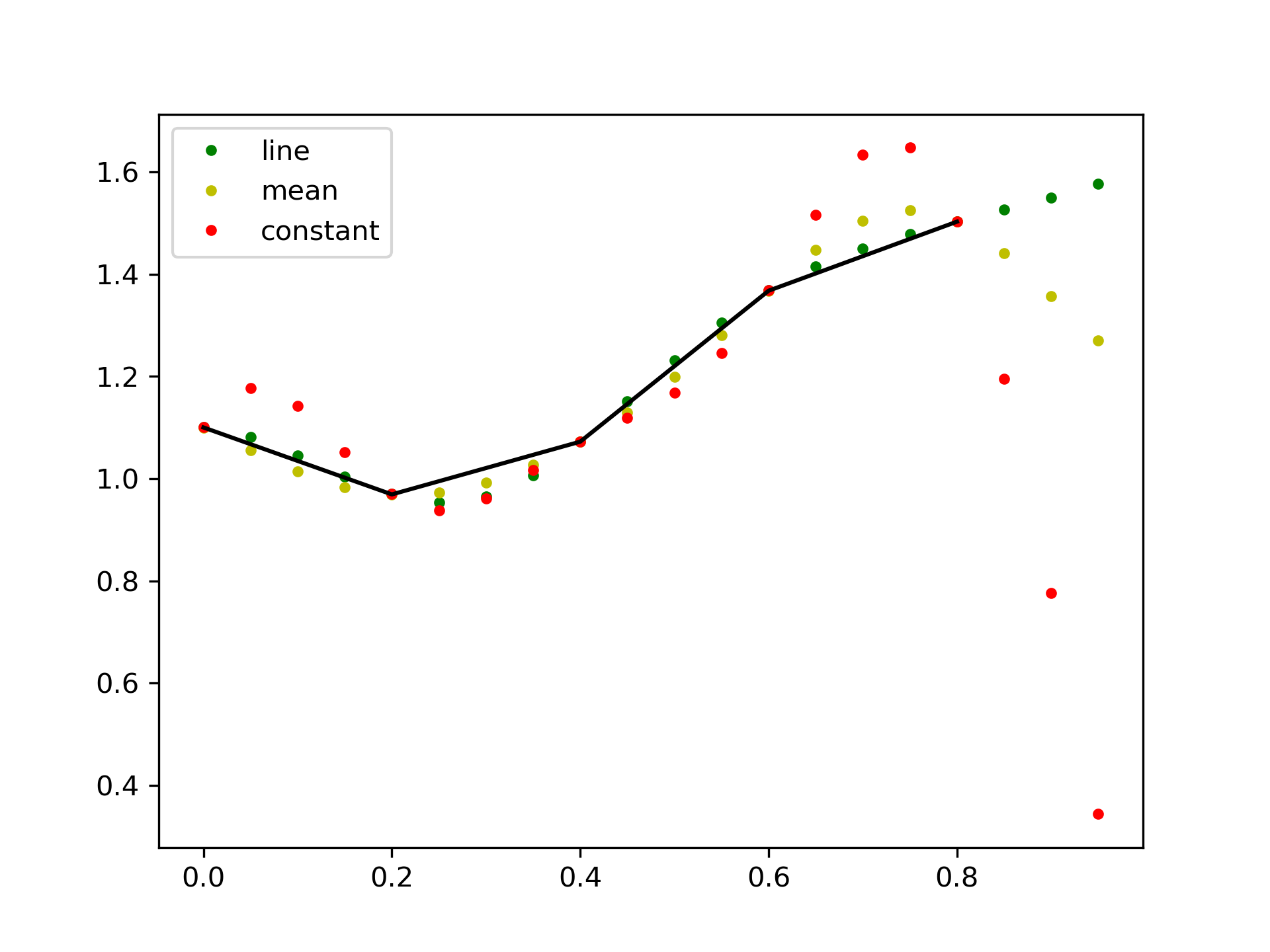
This default behaviour can be changed by using the padtype option:
>>> import numpy as np
... from scipy import signal
>>> N = 5
... x = np.linspace(0, 1, N, endpoint=False)
... y = 2 + x**2 - 1.7*np.sin(x) + .2*np.cos(11*x)
... y2 = 1 + x**3 + 0.1*np.sin(x) + .1*np.cos(11*x)
... Y = np.stack([y, y2], axis=-1)
... up = 4
... xr = np.linspace(0, 1, N*up, endpoint=False)
>>> y2 = signal.resample_poly(Y, up, 1, padtype='constant')
... y3 = signal.resample_poly(Y, up, 1, padtype='mean')
... y4 = signal.resample_poly(Y, up, 1, padtype='line')
>>> import matplotlib.pyplot as plt
... for i in [0,1]:
...     plt.figure()
...     plt.plot(xr, y4[:,i], 'g.', label='line')
...     plt.plot(xr, y3[:,i], 'y.', label='mean')
...     plt.plot(xr, y2[:,i], 'r.', label='constant')
...     plt.plot(x, Y[:,i], 'k-')
...     plt.legend()
... plt.show()
The following pages refer to to this document either explicitly or contain code examples using this.
scipy.signal._signaltools.decimate
scipy.signal._signaltools.resample
scipy.signal._signaltools.resample_poly
Hover to see nodes names; edges to Self not shown, Caped at 50 nodes.
Using a canvas is more power efficient and can get hundred of nodes ; but does not allow hyperlinks; , arrows or text (beyond on hover)
SVG is more flexible but power hungry; and does not scale well to 50 + nodes.
All aboves nodes referred to, (or are referred from) current nodes; Edges from Self to other have been omitted (or all nodes would be connected to the central node "self" which is not useful). Nodes are colored by the library they belong to, and scaled with the number of references pointing them