welch(x, fs=1.0, window='hann', nperseg=None, noverlap=None, nfft=None, detrend='constant', return_onesided=True, scaling='density', axis=-1, average='mean')
Welch's method computes an estimate of the power spectral density by dividing the data into overlapping segments, computing a modified periodogram for each segment and averaging the periodograms.
An appropriate amount of overlap will depend on the choice of window and on your requirements. For the default Hann window an overlap of 50% is a reasonable trade off between accurately estimating the signal power, while not over counting any of the data. Narrower windows may require a larger overlap.
If :None:None:`noverlap` is 0, this method is equivalent to Bartlett's method .
Time series of measurement values
Sampling frequency of the x time series. Defaults to 1.0.
Desired window to use. If :None:None:`window` is a string or tuple, it is passed to get_window
to generate the window values, which are DFT-even by default. See get_window
for a list of windows and required parameters. If :None:None:`window` is array_like it will be used directly as the window and its length must be nperseg. Defaults to a Hann window.
Length of each segment. Defaults to None, but if window is str or tuple, is set to 256, and if window is array_like, is set to the length of the window.
Number of points to overlap between segments. If :None:None:`None`, noverlap = nperseg // 2
. Defaults to :None:None:`None`.
Length of the FFT used, if a zero padded FFT is desired. If :None:None:`None`, the FFT length is :None:None:`nperseg`. Defaults to :None:None:`None`.
Specifies how to detrend each segment. If detrend
is a string, it is passed as the :None:None:`type` argument to the detrend
function. If it is a function, it takes a segment and returns a detrended segment. If detrend
is :None:None:`False`, no detrending is done. Defaults to 'constant'.
If :None:None:`True`, return a one-sided spectrum for real data. If :None:None:`False` return a two-sided spectrum. Defaults to :None:None:`True`, but for complex data, a two-sided spectrum is always returned.
Selects between computing the power spectral density ('density') where :None:None:`Pxx` has units of V**2/Hz and computing the power spectrum ('spectrum') where :None:None:`Pxx` has units of V**2, if x is measured in V and :None:None:`fs` is measured in Hz. Defaults to 'density'
Axis along which the periodogram is computed; the default is over the last axis (i.e. axis=-1
).
Method to use when averaging periodograms. Defaults to 'mean'.
Array of sample frequencies.
Power spectral density or power spectrum of x.
Estimate power spectral density using Welch's method.
lombscargle
Lomb-Scargle periodogram for unevenly sampled data
periodogram
Simple, optionally modified periodogram
>>> from scipy import signal
... import matplotlib.pyplot as plt
... rng = np.random.default_rng()
Generate a test signal, a 2 Vrms sine wave at 1234 Hz, corrupted by 0.001 V**2/Hz of white noise sampled at 10 kHz.
>>> fs = 10e3
... N = 1e5
... amp = 2*np.sqrt(2)
... freq = 1234.0
... noise_power = 0.001 * fs / 2
... time = np.arange(N) / fs
... x = amp*np.sin(2*np.pi*freq*time)
... x += rng.normal(scale=np.sqrt(noise_power), size=time.shape)
Compute and plot the power spectral density.
>>> f, Pxx_den = signal.welch(x, fs, nperseg=1024)
... plt.semilogy(f, Pxx_den)
... plt.ylim([0.5e-3, 1])
... plt.xlabel('frequency [Hz]')
... plt.ylabel('PSD [V**2/Hz]')
... plt.show()
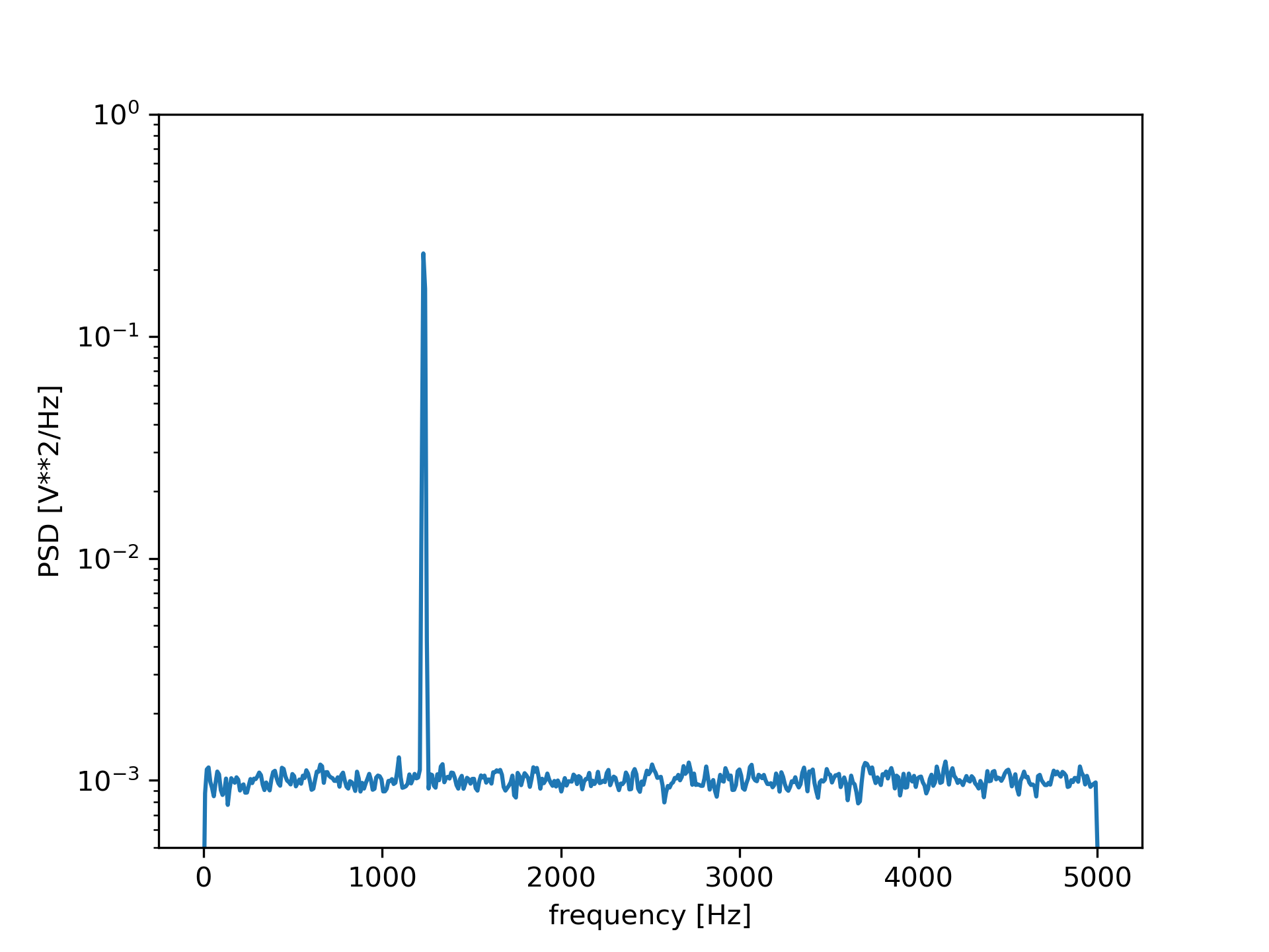
If we average the last half of the spectral density, to exclude the peak, we can recover the noise power on the signal.
>>> np.mean(Pxx_den[256:])
0.0009924865443739191
Now compute and plot the power spectrum.
>>> f, Pxx_spec = signal.welch(x, fs, 'flattop', 1024, scaling='spectrum')
... plt.figure()
... plt.semilogy(f, np.sqrt(Pxx_spec))
... plt.xlabel('frequency [Hz]')
... plt.ylabel('Linear spectrum [V RMS]')
... plt.show()
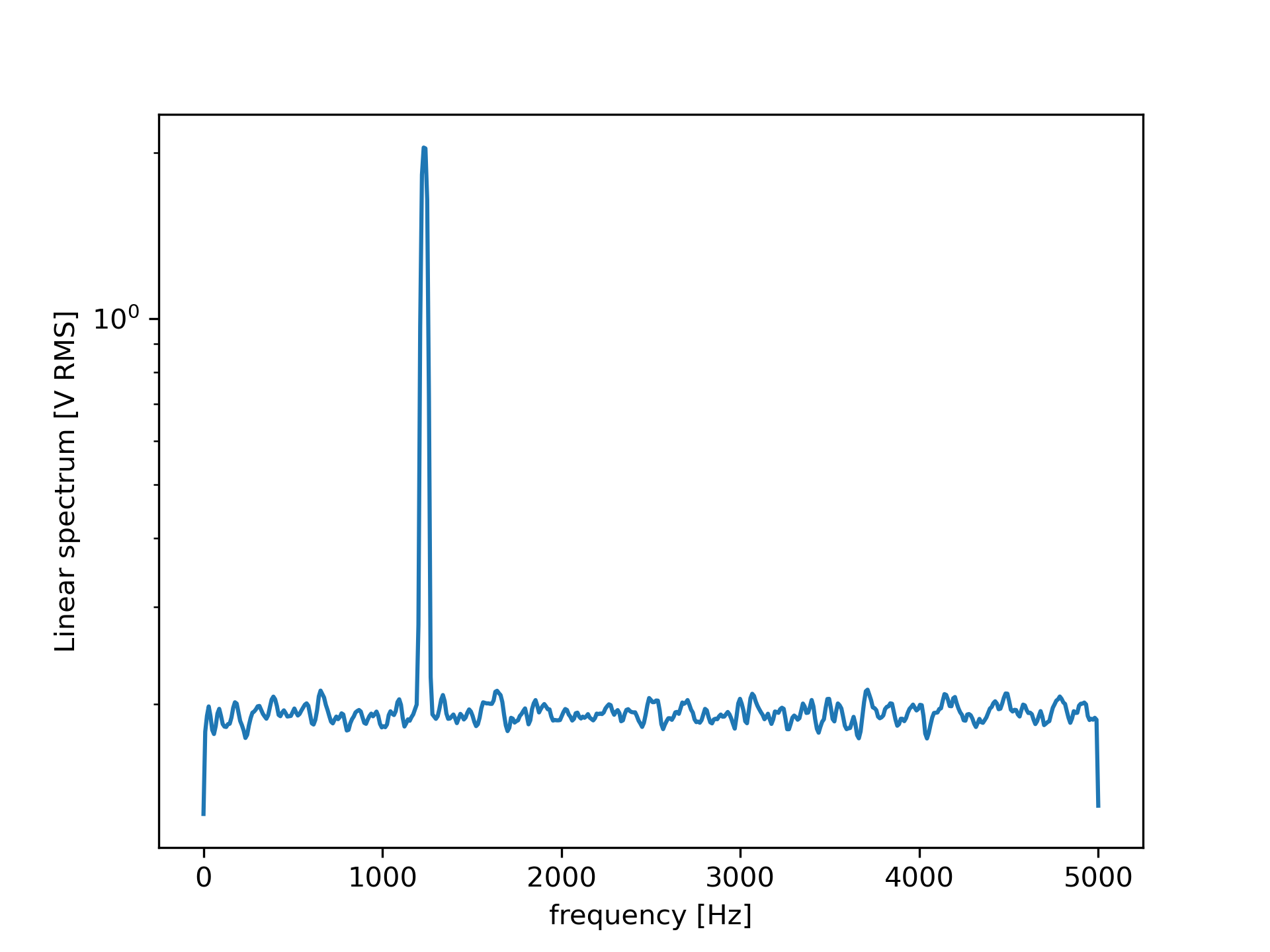
The peak height in the power spectrum is an estimate of the RMS amplitude.
>>> np.sqrt(Pxx_spec.max())
2.0077340678640727
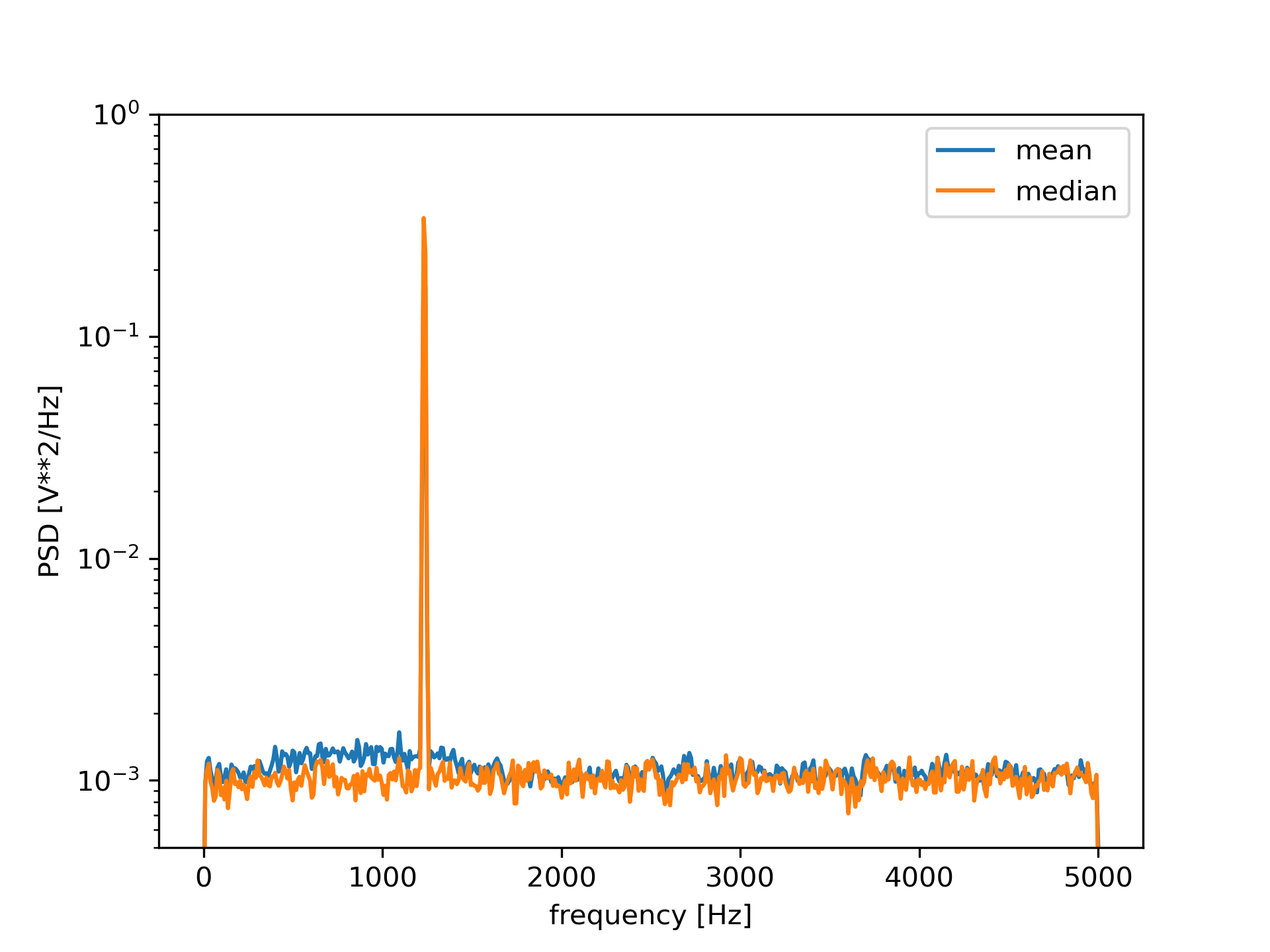
If we now introduce a discontinuity in the signal, by increasing the amplitude of a small portion of the signal by 50, we can see the corruption of the mean average power spectral density, but using a median average better estimates the normal behaviour.
>>> x[int(N//2):int(N//2)+10] *= 50.
... f, Pxx_den = signal.welch(x, fs, nperseg=1024)
... f_med, Pxx_den_med = signal.welch(x, fs, nperseg=1024, average='median')
... plt.semilogy(f, Pxx_den, label='mean')
... plt.semilogy(f_med, Pxx_den_med, label='median')
... plt.ylim([0.5e-3, 1])
... plt.xlabel('frequency [Hz]')
... plt.ylabel('PSD [V**2/Hz]')
... plt.legend()
... plt.show()
The following pages refer to to this document either explicitly or contain code examples using this.
scipy.signal._spectral_py.welch
scipy.signal._spectral_py.coherence
scipy.misc._common.electrocardiogram
scipy.signal._spectral_py.stft
scipy.signal._spectral_py.csd
scipy.signal._spectral_py.periodogram
scipy.signal._spectral_py.spectrogram
scipy.signal._spectral_py.lombscargle
Hover to see nodes names; edges to Self not shown, Caped at 50 nodes.
Using a canvas is more power efficient and can get hundred of nodes ; but does not allow hyperlinks; , arrows or text (beyond on hover)
SVG is more flexible but power hungry; and does not scale well to 50 + nodes.
All aboves nodes referred to, (or are referred from) current nodes; Edges from Self to other have been omitted (or all nodes would be connected to the central node "self" which is not useful). Nodes are colored by the library they belong to, and scaled with the number of references pointing them