lombscargle(x, y, freqs)

The Lomb-Scargle periodogram was developed by Lomb and further extended by Scargle to find, and test the significance of weak periodic signals with uneven temporal sampling.

When normalize is False (default) the computed periodogram is unnormalized, it takes the value (A**2) * N/4 for a harmonic signal with amplitude A for sufficiently large N.

When normalize is True the computed periodogram is normalized by the residuals of the data around a constant reference model (at zero).

Input arrays should be 1-D and will be cast to float64.

Notes

This subroutine calculates the periodogram using a slightly modified algorithm due to Townsend which allows the periodogram to be calculated using only a single pass through the input arrays for each frequency.

The algorithm running time scales roughly as O(x * freqs) or O(N^2) for a large number of samples and frequencies.

Parameters

x : array_like

Sample times.

y : array_like

Measurement values.

freqs : array_like

Angular frequencies for output periodogram.

precenter : bool, optional

Pre-center measurement values by subtracting the mean.

normalize : bool, optional

Compute normalized periodogram.

Raises

ValueError

If the input arrays x and y do not have the same shape.

Returns

pgram : array_like

Lomb-Scargle periodogram.

Computes the Lomb-Scargle periodogram.

See Also

check_COLA

Check whether the Constant OverLap Add (COLA) constraint is met

csd

Cross spectral density by Welch's method

istft

Inverse Short Time Fourier Transform

spectrogram

Spectrogram by Welch's method

welch

Power spectral density by Welch's method

Examples

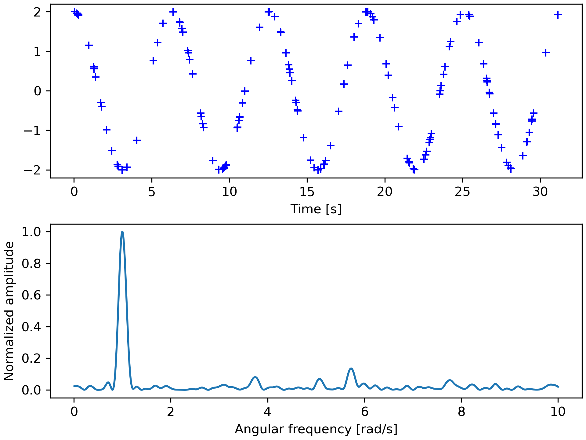
>>> import matplotlib.pyplot as plt
... rng = np.random.default_rng()

First define some input parameters for the signal:

>>> A = 2.
... w0 = 1.  # rad/sec
... nin = 150
... nout = 100000

Randomly generate sample times:

>>> x = rng.uniform(0, 10*np.pi, nin)

Plot a sine wave for the selected times:

>>> y = A * np.cos(w0*x)

Define the array of frequencies for which to compute the periodogram:

>>> w = np.linspace(0.01, 10, nout)

Calculate Lomb-Scargle periodogram:

>>> import scipy.signal as signal
... pgram = signal.lombscargle(x, y, w, normalize=True)

Now make a plot of the input data:

>>> fig, (ax_t, ax_w) = plt.subplots(2, 1, constrained_layout=True)
... ax_t.plot(x, y, 'b+')
... ax_t.set_xlabel('Time [s]')

Then plot the normalized periodogram:

>>> ax_w.plot(w, pgram)
... ax_w.set_xlabel('Angular frequency [rad/s]')
... ax_w.set_ylabel('Normalized amplitude')
... plt.show()

See :

Back References

The following pages refer to to this document either explicitly or contain code examples using this.

scipy.signal._spectral_py.welch scipy.signal._spectral_py.coherence scipy.signal._spectral._lombscargle scipy.signal._spectral_py.stft scipy.signal._spectral_py.csd scipy.signal._spectral_py.periodogram scipy.signal._spectral_py.spectrogram scipy.signal._spectral_py.lombscargle

Local connectivity graph

Hover to see nodes names; edges to Self not shown, Caped at 50 nodes.

Using a canvas is more power efficient and can get hundred of nodes ; but does not allow hyperlinks; , arrows or text (beyond on hover)

SVG is more flexible but power hungry; and does not scale well to 50 + nodes.

All aboves nodes referred to, (or are referred from) current nodes; Edges from Self to other have been omitted (or all nodes would be connected to the central node "self" which is not useful). Nodes are colored by the library they belong to, and scaled with the number of references pointing them

---

GitHub : /scipy/signal/_spectral_py.py#17
type: <class 'function'>
Commit: