spectrogram(x, fs=1.0, window=('tukey', 0.25), nperseg=None, noverlap=None, nfft=None, detrend='constant', return_onesided=True, scaling='density', axis=-1, mode='psd')
Spectrograms can be used as a way of visualizing the change of a nonstationary signal's frequency content over time.
An appropriate amount of overlap will depend on the choice of window and on your requirements. In contrast to welch's method, where the entire data stream is averaged over, one may wish to use a smaller overlap (or perhaps none at all) when computing a spectrogram, to maintain some statistical independence between individual segments. It is for this reason that the default window is a Tukey window with 1/8th of a window's length overlap at each end.
Time series of measurement values
Sampling frequency of the x time series. Defaults to 1.0.
Desired window to use. If :None:None:`window` is a string or tuple, it is passed to get_window
to generate the window values, which are DFT-even by default. See get_window
for a list of windows and required parameters. If :None:None:`window` is array_like it will be used directly as the window and its length must be nperseg. Defaults to a Tukey window with shape parameter of 0.25.
Length of each segment. Defaults to None, but if window is str or tuple, is set to 256, and if window is array_like, is set to the length of the window.
Number of points to overlap between segments. If :None:None:`None`, noverlap = nperseg // 8
. Defaults to :None:None:`None`.
Length of the FFT used, if a zero padded FFT is desired. If :None:None:`None`, the FFT length is :None:None:`nperseg`. Defaults to :None:None:`None`.
Specifies how to detrend each segment. If detrend
is a string, it is passed as the :None:None:`type` argument to the detrend
function. If it is a function, it takes a segment and returns a detrended segment. If detrend
is :None:None:`False`, no detrending is done. Defaults to 'constant'.
If :None:None:`True`, return a one-sided spectrum for real data. If :None:None:`False` return a two-sided spectrum. Defaults to :None:None:`True`, but for complex data, a two-sided spectrum is always returned.
Selects between computing the power spectral density ('density') where :None:None:`Sxx` has units of V**2/Hz and computing the power spectrum ('spectrum') where :None:None:`Sxx` has units of V**2, if x is measured in V and :None:None:`fs` is measured in Hz. Defaults to 'density'.
Axis along which the spectrogram is computed; the default is over the last axis (i.e. axis=-1
).
Defines what kind of return values are expected. Options are ['psd', 'complex', 'magnitude', 'angle', 'phase']. 'complex' is equivalent to the output of stft
with no padding or boundary extension. 'magnitude' returns the absolute magnitude of the STFT. 'angle' and 'phase' return the complex angle of the STFT, with and without unwrapping, respectively.
Array of sample frequencies.
Array of segment times.
Spectrogram of x. By default, the last axis of Sxx corresponds to the segment times.
Compute a spectrogram with consecutive Fourier transforms.
csd
Cross spectral density by Welch's method.
lombscargle
Lomb-Scargle periodogram for unevenly sampled data
periodogram
Simple, optionally modified periodogram
welch
Power spectral density by Welch's method.
>>> from scipy import signal
... from scipy.fft import fftshift
... import matplotlib.pyplot as plt
... rng = np.random.default_rng()
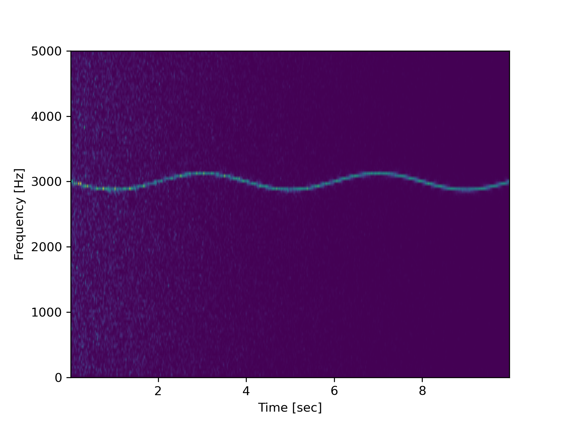
Generate a test signal, a 2 Vrms sine wave whose frequency is slowly modulated around 3kHz, corrupted by white noise of exponentially decreasing magnitude sampled at 10 kHz.
>>> fs = 10e3
... N = 1e5
... amp = 2 * np.sqrt(2)
... noise_power = 0.01 * fs / 2
... time = np.arange(N) / float(fs)
... mod = 500*np.cos(2*np.pi*0.25*time)
... carrier = amp * np.sin(2*np.pi*3e3*time + mod)
... noise = rng.normal(scale=np.sqrt(noise_power), size=time.shape)
... noise *= np.exp(-time/5)
... x = carrier + noise
Compute and plot the spectrogram.
>>> f, t, Sxx = signal.spectrogram(x, fs)
... plt.pcolormesh(t, f, Sxx, shading='gouraud')
... plt.ylabel('Frequency [Hz]')
... plt.xlabel('Time [sec]')
... plt.show()
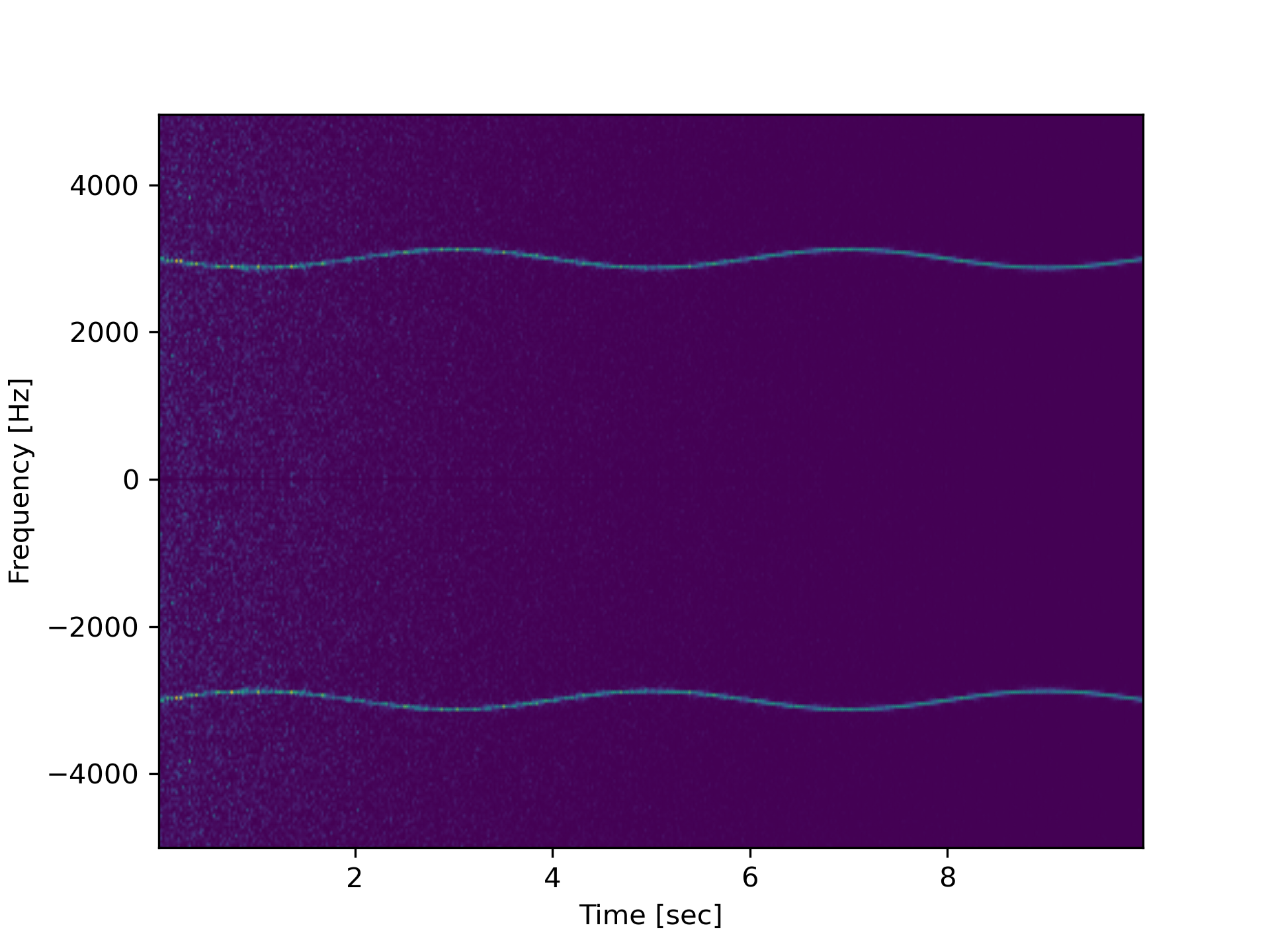
Note, if using output that is not one sided, then use the following:
>>> f, t, Sxx = signal.spectrogram(x, fs, return_onesided=False)
... plt.pcolormesh(t, fftshift(f), fftshift(Sxx, axes=0), shading='gouraud')
... plt.ylabel('Frequency [Hz]')
... plt.xlabel('Time [sec]')
... plt.show()
The following pages refer to to this document either explicitly or contain code examples using this.
scipy.signal._spectral_py.stft
scipy.signal._spectral_py.spectrogram
scipy.signal._waveforms.chirp
scipy.signal._spectral_py.lombscargle
Hover to see nodes names; edges to Self not shown, Caped at 50 nodes.
Using a canvas is more power efficient and can get hundred of nodes ; but does not allow hyperlinks; , arrows or text (beyond on hover)
SVG is more flexible but power hungry; and does not scale well to 50 + nodes.
All aboves nodes referred to, (or are referred from) current nodes; Edges from Self to other have been omitted (or all nodes would be connected to the central node "self" which is not useful). Nodes are colored by the library they belong to, and scaled with the number of references pointing them