sosfreqz(sos, worN=512, whole=False, fs=6.283185307179586)
Given :None:None:`sos`, an array with shape (n, 6) of second order sections of a digital filter, compute the frequency response of the system function:
       B0(z)   B1(z)         B{n-1}(z)
H(z) = ----- * ----- * ... * ---------
       A0(z)   A1(z)         A{n-1}(z)
for z = exp(omega*1j), where B{k}(z) and A{k}(z) are numerator and denominator of the transfer function of the k-th second order section.
Array of second-order filter coefficients, must have shape (n_sections, 6)
. Each row corresponds to a second-order section, with the first three columns providing the numerator coefficients and the last three providing the denominator coefficients.
If a single integer, then compute at that many frequencies (default is N=512). Using a number that is fast for FFT computations can result in faster computations (see Notes of freqz
).
If an array_like, compute the response at the frequencies given (must be 1-D). These are in the same units as :None:None:`fs`.
Normally, frequencies are computed from 0 to the Nyquist frequency, fs/2 (upper-half of unit-circle). If :None:None:`whole` is True, compute frequencies from 0 to fs.
The sampling frequency of the digital system. Defaults to 2*pi radians/sample (so w is from 0 to pi).
The frequencies at which h was computed, in the same units as :None:None:`fs`. By default, w is normalized to the range [0, pi) (radians/sample).
The frequency response, as complex numbers.
Compute the frequency response of a digital filter in SOS format.
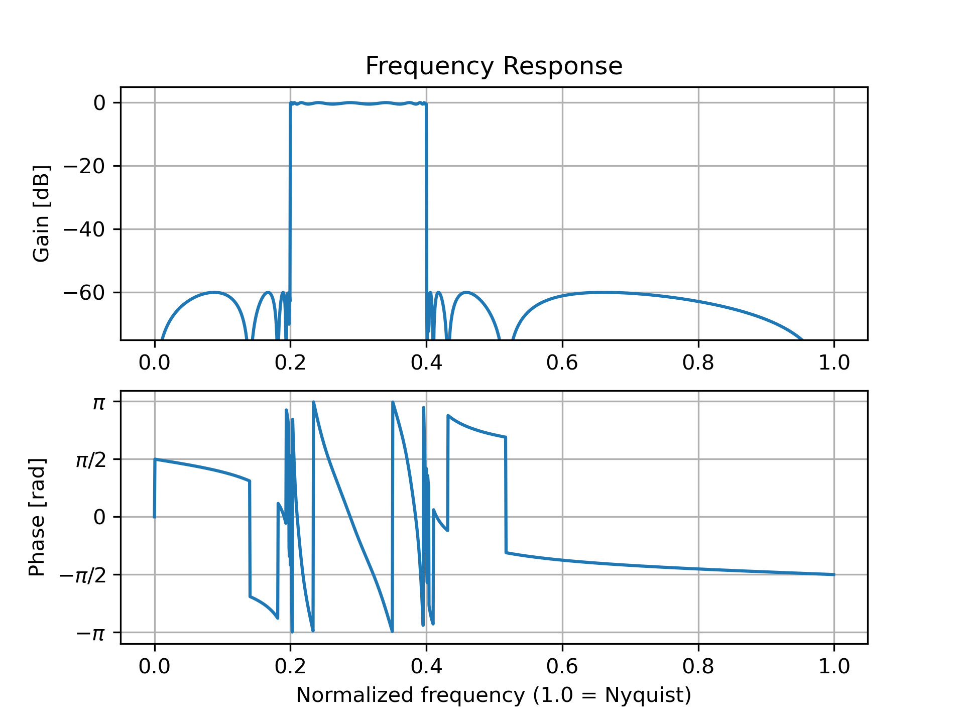
Design a 15th-order bandpass filter in SOS format.
>>> from scipy import signal
... sos = signal.ellip(15, 0.5, 60, (0.2, 0.4), btype='bandpass',
...                    output='sos')
Compute the frequency response at 1500 points from DC to Nyquist.
>>> w, h = signal.sosfreqz(sos, worN=1500)
Plot the response.
>>> import matplotlib.pyplot as plt
... plt.subplot(2, 1, 1)
... db = 20*np.log10(np.maximum(np.abs(h), 1e-5))
... plt.plot(w/np.pi, db)
... plt.ylim(-75, 5)
... plt.grid(True)
... plt.yticks([0, -20, -40, -60])
... plt.ylabel('Gain [dB]')
... plt.title('Frequency Response')
... plt.subplot(2, 1, 2)
... plt.plot(w/np.pi, np.angle(h))
... plt.grid(True)
... plt.yticks([-np.pi, -0.5*np.pi, 0, 0.5*np.pi, np.pi],
...            [r'$-\pi$', r'$-\pi/2$', '0', r'$\pi/2$', r'$\pi$'])
... plt.ylabel('Phase [rad]')
... plt.xlabel('Normalized frequency (1.0 = Nyquist)')
... plt.show()
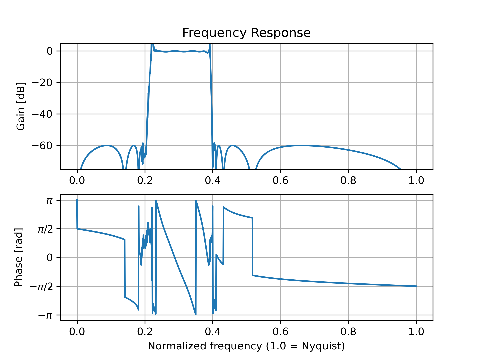
If the same filter is implemented as a single transfer function, numerical error corrupts the frequency response:
>>> b, a = signal.ellip(15, 0.5, 60, (0.2, 0.4), btype='bandpass',
...                    output='ba')
... w, h = signal.freqz(b, a, worN=1500)
... plt.subplot(2, 1, 1)
... db = 20*np.log10(np.maximum(np.abs(h), 1e-5))
... plt.plot(w/np.pi, db)
... plt.ylim(-75, 5)
... plt.grid(True)
... plt.yticks([0, -20, -40, -60])
... plt.ylabel('Gain [dB]')
... plt.title('Frequency Response')
... plt.subplot(2, 1, 2)
... plt.plot(w/np.pi, np.angle(h))
... plt.grid(True)
... plt.yticks([-np.pi, -0.5*np.pi, 0, 0.5*np.pi, np.pi],
...            [r'$-\pi$', r'$-\pi/2$', '0', r'$\pi/2$', r'$\pi$'])
... plt.ylabel('Phase [rad]')
... plt.xlabel('Normalized frequency (1.0 = Nyquist)')
... plt.show()
The following pages refer to to this document either explicitly or contain code examples using this.
scipy.signal._signaltools.sosfiltfilt
scipy.signal._filter_design.iirfilter
scipy.signal._filter_design.sosfreqz
scipy.signal._signaltools.sosfilt
scipy.signal._filter_design.freqz
Hover to see nodes names; edges to Self not shown, Caped at 50 nodes.
Using a canvas is more power efficient and can get hundred of nodes ; but does not allow hyperlinks; , arrows or text (beyond on hover)
SVG is more flexible but power hungry; and does not scale well to 50 + nodes.
All aboves nodes referred to, (or are referred from) current nodes; Edges from Self to other have been omitted (or all nodes would be connected to the central node "self" which is not useful). Nodes are colored by the library they belong to, and scaled with the number of references pointing them