iircomb(w0, Q, ftype='notch', fs=2.0)
A notching comb filter is a band-stop filter with a narrow bandwidth (high quality factor). It rejects a narrow frequency band and leaves the rest of the spectrum little changed.
A peaking comb filter is a band-pass filter with a narrow bandwidth (high quality factor). It rejects components outside a narrow frequency band.
For implementation details, see . The TF implementation of the comb filter is numerically stable even at higher orders due to the use of a single repeated pole, which won't suffer from precision loss.
Frequency to attenuate (notching) or boost (peaking). If :None:None:`fs` is specified, this is in the same units as :None:None:`fs`. By default, it is a normalized scalar that must satisfy 0 < w0 < 1
, with w0 = 1
corresponding to half of the sampling frequency.
Quality factor. Dimensionless parameter that characterizes notch filter -3 dB bandwidth bw
relative to its center frequency, Q = w0/bw
.
The type of comb filter generated by the function. If 'notch', then it returns a filter with notches at frequencies 0
, w0
, 2 * w0
, etc. If 'peak', then it returns a filter with peaks at frequencies 0.5 * w0
, 1.5 * w0
, 2.5 * w0`
, etc. Default is 'notch'.
The sampling frequency of the signal. Default is 2.0.
If :None:None:`w0` is less than or equal to 0 or greater than or equal to fs/2
, if :None:None:`fs` is not divisible by :None:None:`w0`, if :None:None:`ftype` is not 'notch' or 'peak'
Numerator ( b
) and denominator ( a
) polynomials of the IIR filter.
Design IIR notching or peaking digital comb filter.
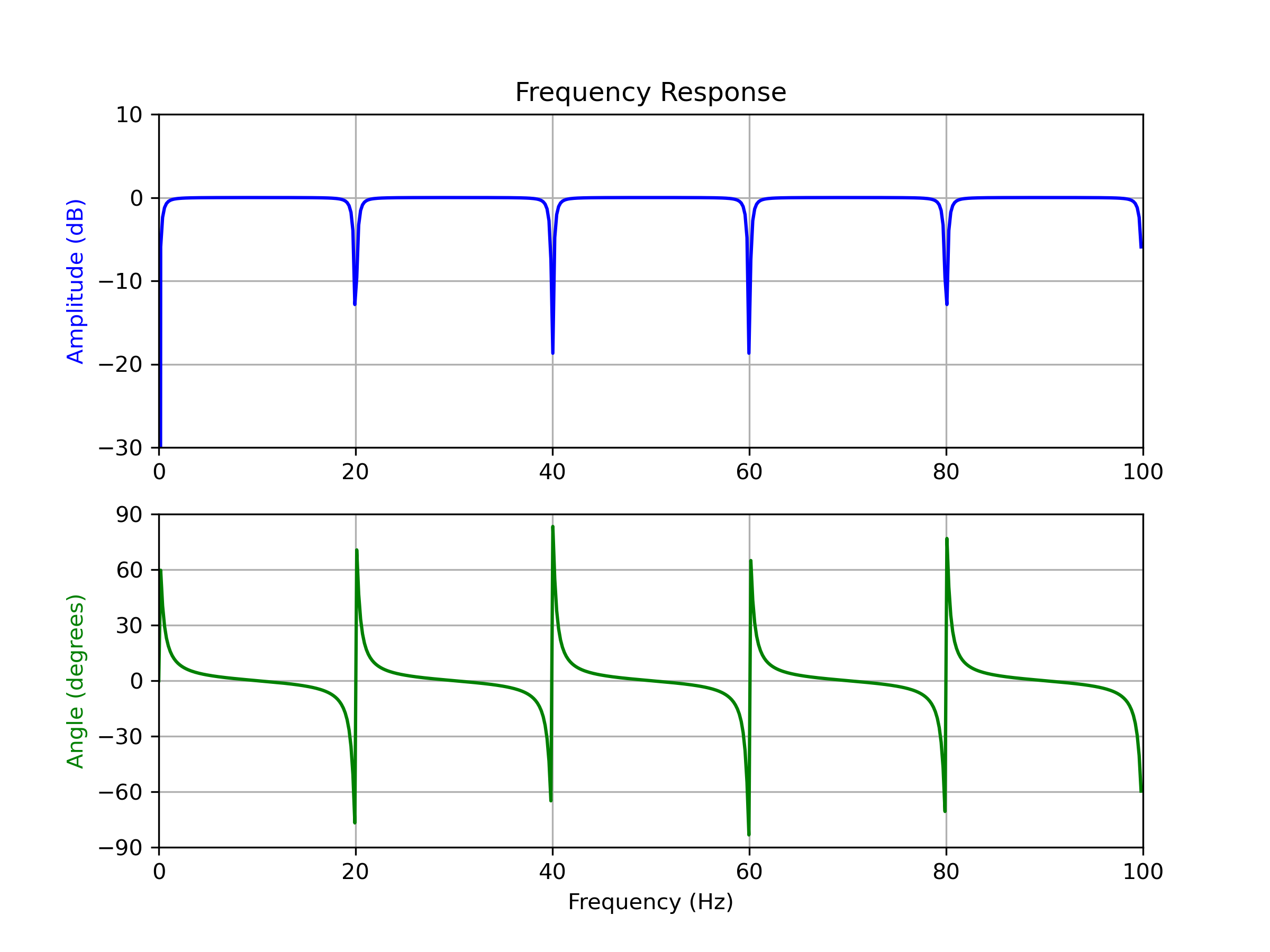
Design and plot notching comb filter at 20 Hz for a signal sampled at 200 Hz, using quality factor Q = 30
>>> from scipy import signal
... import matplotlib.pyplot as plt
>>> fs = 200.0  # Sample frequency (Hz)
... f0 = 20.0  # Frequency to be removed from signal (Hz)
... Q = 30.0  # Quality factor
... # Design notching comb filter
... b, a = signal.iircomb(f0, Q, ftype='notch', fs=fs)
>>> # Frequency response
... freq, h = signal.freqz(b, a, fs=fs)
... response = abs(h)
... # To avoid divide by zero when graphing
... response[response == 0] = 1e-20
... # Plot
... fig, ax = plt.subplots(2, 1, figsize=(8, 6))
... ax[0].plot(freq, 20*np.log10(abs(response)), color='blue')
... ax[0].set_title("Frequency Response")
... ax[0].set_ylabel("Amplitude (dB)", color='blue')
... ax[0].set_xlim([0, 100])
... ax[0].set_ylim([-30, 10])
... ax[0].grid()
... ax[1].plot(freq, np.unwrap(np.angle(h))*180/np.pi, color='green')
... ax[1].set_ylabel("Angle (degrees)", color='green')
... ax[1].set_xlabel("Frequency (Hz)")
... ax[1].set_xlim([0, 100])
... ax[1].set_yticks([-90, -60, -30, 0, 30, 60, 90])
... ax[1].set_ylim([-90, 90])
... ax[1].grid()
... plt.show()
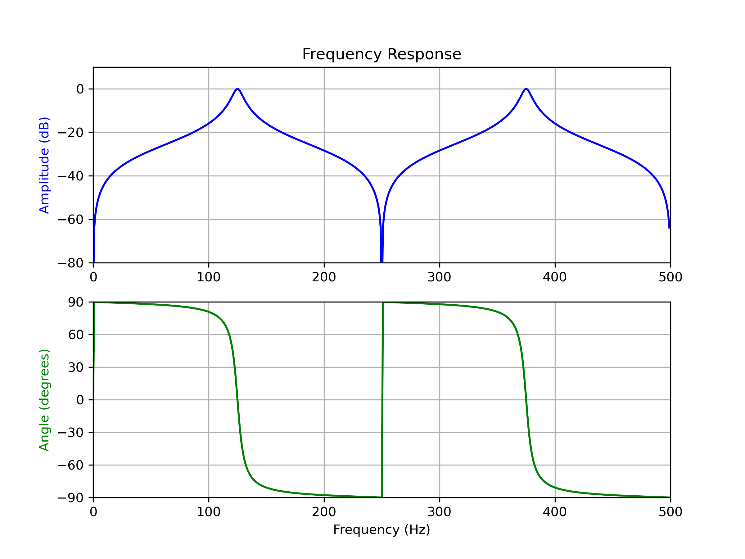
Design and plot peaking comb filter at 250 Hz for a signal sampled at 1000 Hz, using quality factor Q = 30
>>> fs = 1000.0  # Sample frequency (Hz)
... f0 = 250.0  # Frequency to be retained (Hz)
... Q = 30.0  # Quality factor
... # Design peaking filter
... b, a = signal.iircomb(f0, Q, ftype='peak', fs=fs)
>>> # Frequency response
... freq, h = signal.freqz(b, a, fs=fs)
... response = abs(h)
... # To avoid divide by zero when graphing
... response[response == 0] = 1e-20
... # Plot
... fig, ax = plt.subplots(2, 1, figsize=(8, 6))
... ax[0].plot(freq, 20*np.log10(np.maximum(abs(h), 1e-5)), color='blue')
... ax[0].set_title("Frequency Response")
... ax[0].set_ylabel("Amplitude (dB)", color='blue')
... ax[0].set_xlim([0, 500])
... ax[0].set_ylim([-80, 10])
... ax[0].grid()
... ax[1].plot(freq, np.unwrap(np.angle(h))*180/np.pi, color='green')
... ax[1].set_ylabel("Angle (degrees)", color='green')
... ax[1].set_xlabel("Frequency (Hz)")
... ax[1].set_xlim([0, 500])
... ax[1].set_yticks([-90, -60, -30, 0, 30, 60, 90])
... ax[1].set_ylim([-90, 90])
... ax[1].grid()
... plt.show()
The following pages refer to to this document either explicitly or contain code examples using this.
scipy.signal._filter_design.iircomb
Hover to see nodes names; edges to Self not shown, Caped at 50 nodes.
Using a canvas is more power efficient and can get hundred of nodes ; but does not allow hyperlinks; , arrows or text (beyond on hover)
SVG is more flexible but power hungry; and does not scale well to 50 + nodes.
All aboves nodes referred to, (or are referred from) current nodes; Edges from Self to other have been omitted (or all nodes would be connected to the central node "self" which is not useful). Nodes are colored by the library they belong to, and scaled with the number of references pointing them