freqz_zpk(z, p, k, worN=512, whole=False, fs=6.283185307179586)
Given the Zeros, Poles and Gain of a digital filter, compute its frequency response:
$H(z)=k \prod_i (z - Z[i]) / \prod_j (z - P[j])$
where $k$
is the :None:None:`gain`, $Z$
are the zeros
and $P$
are the :None:None:`poles`.
Zeroes of a linear filter
Poles of a linear filter
Gain of a linear filter
If a single integer, then compute at that many frequencies (default is N=512).
If an array_like, compute the response at the frequencies given. These are in the same units as :None:None:`fs`.
Normally, frequencies are computed from 0 to the Nyquist frequency, fs/2 (upper-half of unit-circle). If :None:None:`whole` is True, compute frequencies from 0 to fs. Ignored if w is array_like.
The sampling frequency of the digital system. Defaults to 2*pi radians/sample (so w is from 0 to pi).
The frequencies at which h was computed, in the same units as :None:None:`fs`. By default, w is normalized to the range [0, pi) (radians/sample).
The frequency response, as complex numbers.
Compute the frequency response of a digital filter in ZPK form.
freqs
Compute the frequency response of an analog filter in TF form
freqs_zpk
Compute the frequency response of an analog filter in ZPK form
freqz
Compute the frequency response of a digital filter in TF form
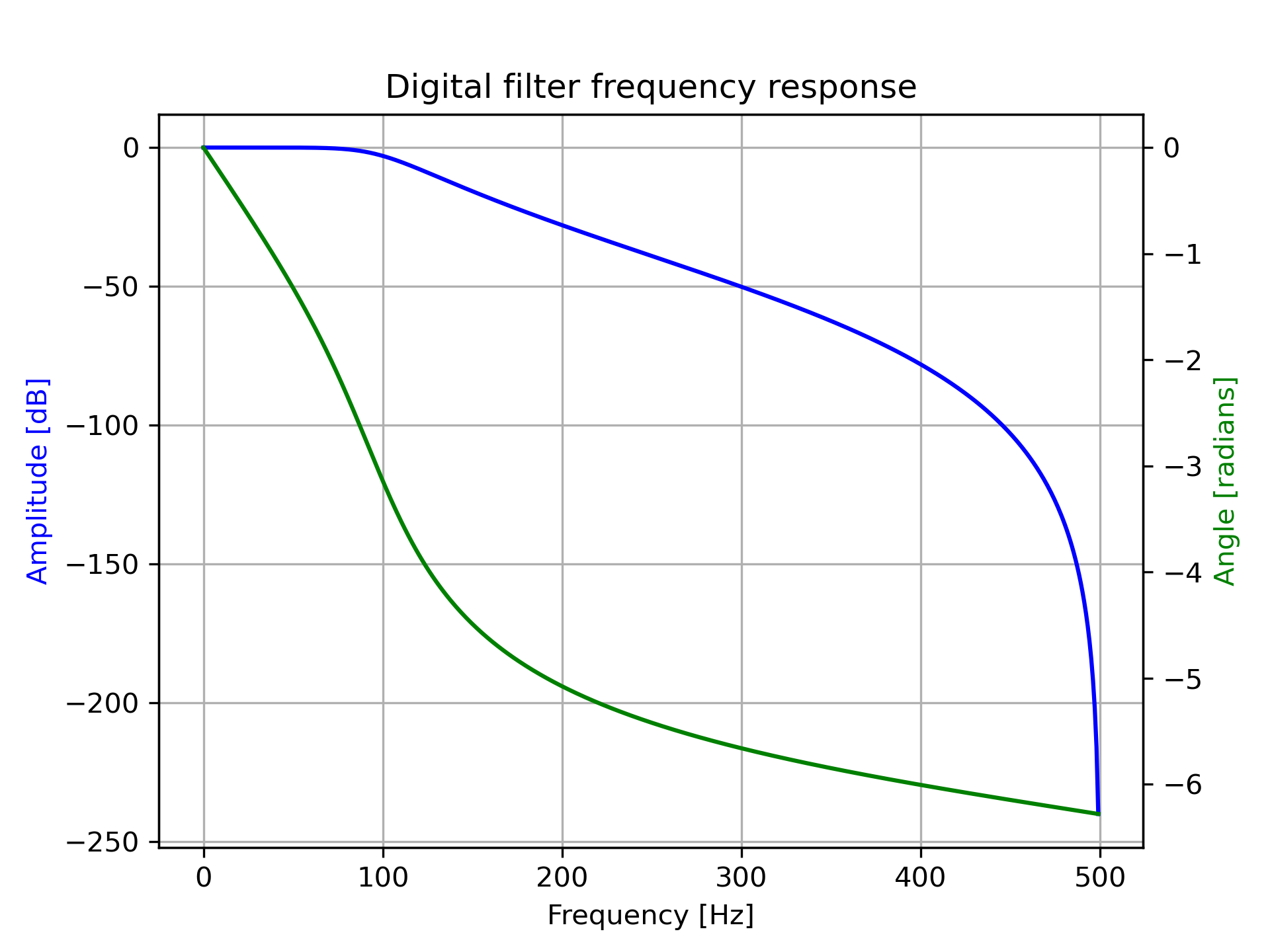
Design a 4th-order digital Butterworth filter with cut-off of 100 Hz in a system with sample rate of 1000 Hz, and plot the frequency response:
>>> from scipy import signal
... z, p, k = signal.butter(4, 100, output='zpk', fs=1000)
... w, h = signal.freqz_zpk(z, p, k, fs=1000)
>>> import matplotlib.pyplot as plt
... fig = plt.figure()
... ax1 = fig.add_subplot(1, 1, 1)
... ax1.set_title('Digital filter frequency response')
>>> ax1.plot(w, 20 * np.log10(abs(h)), 'b')
... ax1.set_ylabel('Amplitude [dB]', color='b')
... ax1.set_xlabel('Frequency [Hz]')
... ax1.grid()
>>> ax2 = ax1.twinx()
... angles = np.unwrap(np.angle(h))
... ax2.plot(w, angles, 'g')
... ax2.set_ylabel('Angle [radians]', color='g')
>>> plt.axis('tight')
... plt.show()
The following pages refer to to this document either explicitly or contain code examples using this.
scipy.signal._filter_design.bilinear_zpk
scipy.signal._filter_design.freqz
scipy.signal._filter_design.freqz_zpk
scipy.signal._filter_design.freqs_zpk
Hover to see nodes names; edges to Self not shown, Caped at 50 nodes.
Using a canvas is more power efficient and can get hundred of nodes ; but does not allow hyperlinks; , arrows or text (beyond on hover)
SVG is more flexible but power hungry; and does not scale well to 50 + nodes.
All aboves nodes referred to, (or are referred from) current nodes; Edges from Self to other have been omitted (or all nodes would be connected to the central node "self" which is not useful). Nodes are colored by the library they belong to, and scaled with the number of references pointing them