Document

scipy 1.8.0 Pypi GitHub Homepage

freqs(b, a, worN=200, plot=None)

Given the M-order numerator b and N-order denominator a of an analog filter, compute its frequency response:

        b[0]*(jw)**M + b[1]*(jw)**(M-1) + ... + b[M]
H(w) = ----------------------------------------------
        a[0]*(jw)**N + a[1]*(jw)**(N-1) + ... + a[N]

Notes

Using Matplotlib's "plot" function as the callable for :None:None:`plot` produces unexpected results, this plots the real part of the complex transfer function, not the magnitude. Try lambda w, h: plot(w, abs(h)) .

Parameters

b : array_like: Numerator of a linear filter.
a : array_like: Denominator of a linear filter.
worN : {None, int, array_like}, optional: If None, then compute at 200 frequencies around the interesting parts of the response curve (determined by pole-zero locations). If a single integer, then compute at that many frequencies. Otherwise, compute the response at the angular frequencies (e.g., rad/s) given in :None:None:`worN`.
plot : callable, optional: A callable that takes two arguments. If given, the return parameters w and h are passed to plot. Useful for plotting the frequency response inside freqs .

Returns

w : ndarray: The angular frequencies at which h was computed.
h : ndarray: The frequency response.

Compute frequency response of analog filter.

Examples

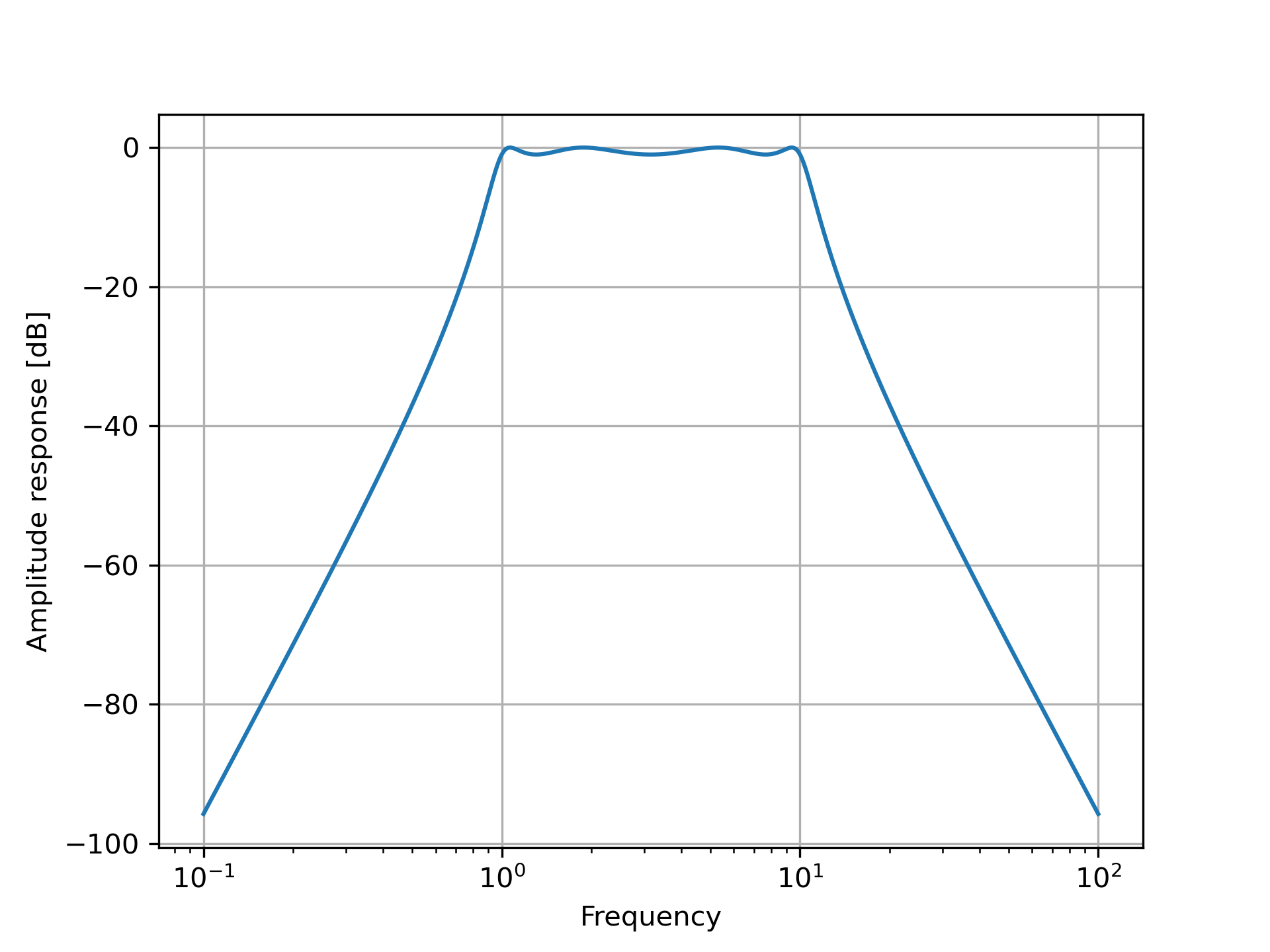
>>> from scipy.signal import freqs, iirfilter

>>> b, a = iirfilter(4, [1, 10], 1, 60, analog=True, ftype='cheby1')

>>> w, h = freqs(b, a, worN=np.logspace(-1, 2, 1000))

>>> import matplotlib.pyplot as plt
... plt.semilogx(w, 20 * np.log10(abs(h)))
... plt.xlabel('Frequency')
... plt.ylabel('Amplitude response [dB]')
... plt.grid()
... plt.show()

See :

Back References

The following pages refer to to this document either explicitly or contain code examples using this.

scipy.signal._filter_design.freqs scipy.signal._filter_design.butter scipy.signal._filter_design.ellip scipy.signal._filter_design.ellipord scipy.signal._filter_design.iirfilter scipy.signal._filter_design.cheby2 scipy.signal._filter_design.freqz_zpk scipy.signal._filter_design.buttord scipy.signal._filter_design.freqs_zpk scipy.signal._filter_design.cheby1 scipy.signal._filter_design.bessel scipy.signal._filter_design.bilinear

Local connectivity graph

Hover to see nodes names; edges to Self not shown, Caped at 50 nodes.

Using a canvas is more power efficient and can get hundred of nodes ; but does not allow hyperlinks; , arrows or text (beyond on hover)

SVG is more flexible but power hungry; and does not scale well to 50 + nodes.

All aboves nodes referred to, (or are referred from) current nodes; Edges from Self to other have been omitted (or all nodes would be connected to the central node "self" which is not useful). Nodes are colored by the library they belong to, and scaled with the number of references pointing them