cheby1(N, rp, Wn, btype='low', analog=False, output='ba', fs=None)
Design an Nth-order digital or analog Chebyshev type I filter and return the filter coefficients.
The Chebyshev type I filter maximizes the rate of cutoff between the frequency response's passband and stopband, at the expense of ripple in the passband and increased ringing in the step response.
Type I filters roll off faster than Type II (cheby2
), but Type II filters do not have any ripple in the passband.
The equiripple passband has N maxima or minima (for example, a 5th-order filter has 3 maxima and 2 minima). Consequently, the DC gain is unity for odd-order filters, or -rp dB for even-order filters.
The 'sos'
output parameter was added in 0.16.0.
The order of the filter.
The maximum ripple allowed below unity gain in the passband. Specified in decibels, as a positive number.
A scalar or length-2 sequence giving the critical frequencies. For Type I filters, this is the point in the transition band at which the gain first drops below -:None:None:`rp`.
For digital filters, :None:None:`Wn` are in the same units as :None:None:`fs`. By default, :None:None:`fs` is 2 half-cycles/sample, so these are normalized from 0 to 1, where 1 is the Nyquist frequency. (:None:None:`Wn` is thus in half-cycles / sample.)
For analog filters, :None:None:`Wn` is an angular frequency (e.g., rad/s).
The type of filter. Default is 'lowpass'.
When True, return an analog filter, otherwise a digital filter is returned.
Type of output: numerator/denominator ('ba'), pole-zero ('zpk'), or second-order sections ('sos'). Default is 'ba' for backwards compatibility, but 'sos' should be used for general-purpose filtering.
The sampling frequency of the digital system.
Numerator (b) and denominator (a) polynomials of the IIR filter. Only returned if output='ba'
.
Zeros, poles, and system gain of the IIR filter transfer function. Only returned if output='zpk'
.
Second-order sections representation of the IIR filter. Only returned if output=='sos'
.
Chebyshev type I digital and analog filter design.
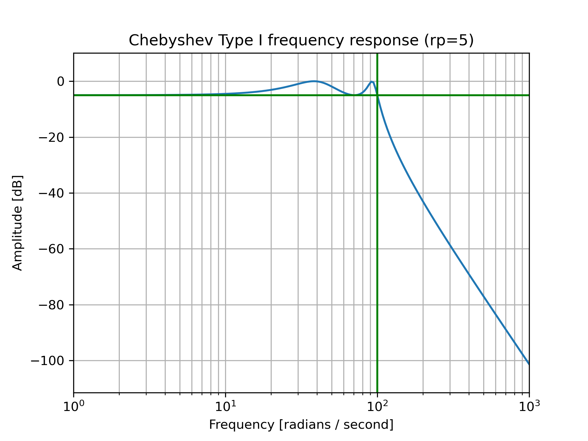
Design an analog filter and plot its frequency response, showing the critical points:
>>> from scipy import signal
... import matplotlib.pyplot as plt
>>> b, a = signal.cheby1(4, 5, 100, 'low', analog=True)
... w, h = signal.freqs(b, a)
... plt.semilogx(w, 20 * np.log10(abs(h)))
... plt.title('Chebyshev Type I frequency response (rp=5)')
... plt.xlabel('Frequency [radians / second]')
... plt.ylabel('Amplitude [dB]')
... plt.margins(0, 0.1)
... plt.grid(which='both', axis='both')
... plt.axvline(100, color='green') # cutoff frequency
... plt.axhline(-5, color='green') # rp
... plt.show()
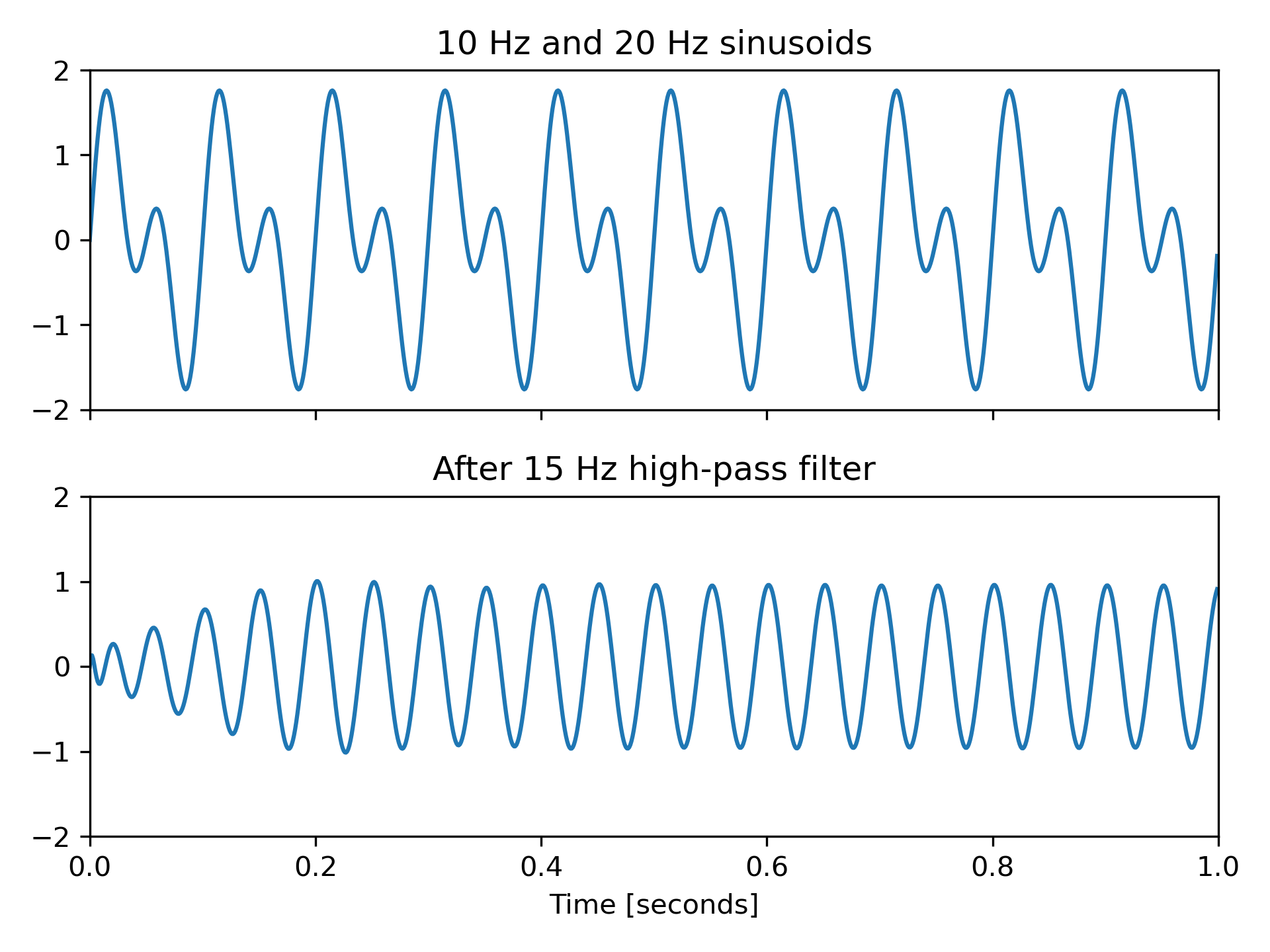
Generate a signal made up of 10 Hz and 20 Hz, sampled at 1 kHz
>>> t = np.linspace(0, 1, 1000, False)  # 1 second
... sig = np.sin(2*np.pi*10*t) + np.sin(2*np.pi*20*t)
... fig, (ax1, ax2) = plt.subplots(2, 1, sharex=True)
... ax1.plot(t, sig)
... ax1.set_title('10 Hz and 20 Hz sinusoids')
... ax1.axis([0, 1, -2, 2])
Design a digital high-pass filter at 15 Hz to remove the 10 Hz tone, and apply it to the signal. (It's recommended to use second-order sections format when filtering, to avoid numerical error with transfer function ( ba
) format):
>>> sos = signal.cheby1(10, 1, 15, 'hp', fs=1000, output='sos')
... filtered = signal.sosfilt(sos, sig)
... ax2.plot(t, filtered)
... ax2.set_title('After 15 Hz high-pass filter')
... ax2.axis([0, 1, -2, 2])
... ax2.set_xlabel('Time [seconds]')
... plt.tight_layout()
... plt.show()
The following pages refer to to this document either explicitly or contain code examples using this.
scipy.signal._filter_design.ellip
scipy.signal._filter_design.iirfilter
scipy.signal._filter_design.cheb1ap
scipy.signal._filter_design.cheby2
scipy.signal._filter_design.cheb1ord
scipy.signal._filter_design.cheby1
scipy.signal._filter_design.iirdesign
Hover to see nodes names; edges to Self not shown, Caped at 50 nodes.
Using a canvas is more power efficient and can get hundred of nodes ; but does not allow hyperlinks; , arrows or text (beyond on hover)
SVG is more flexible but power hungry; and does not scale well to 50 + nodes.
All aboves nodes referred to, (or are referred from) current nodes; Edges from Self to other have been omitted (or all nodes would be connected to the central node "self" which is not useful). Nodes are colored by the library they belong to, and scaled with the number of references pointing them