buttord(wp, ws, gpass, gstop, analog=False, fs=None)
Return the order of the lowest order digital or analog Butterworth filter that loses no more than gpass
dB in the passband and has at least gstop
dB attenuation in the stopband.
Passband and stopband edge frequencies.
For digital filters, these are in the same units as :None:None:`fs`. By default, :None:None:`fs` is 2 half-cycles/sample, so these are normalized from 0 to 1, where 1 is the Nyquist frequency. (:None:None:`wp` and :None:None:`ws` are thus in half-cycles / sample.) For example:
Lowpass: wp = 0.2, ws = 0.3
Highpass: wp = 0.3, ws = 0.2
Bandpass: wp = [0.2, 0.5], ws = [0.1, 0.6]
Bandstop: wp = [0.1, 0.6], ws = [0.2, 0.5]
For analog filters, :None:None:`wp` and :None:None:`ws` are angular frequencies (e.g., rad/s).
The maximum loss in the passband (dB).
The minimum attenuation in the stopband (dB).
When True, return an analog filter, otherwise a digital filter is returned.
The sampling frequency of the digital system.
The lowest order for a Butterworth filter which meets specs.
The Butterworth natural frequency (i.e. the "3dB frequency"). Should be used with butter
to give filter results. If :None:None:`fs` is specified, this is in the same units, and :None:None:`fs` must also be passed to butter
.
Butterworth filter order selection.
butter
Filter design using order and critical points
cheb1ord
Find order and critical points from passband and stopband spec
iirdesign
General filter design using passband and stopband spec
iirfilter
General filter design using order and critical frequencies
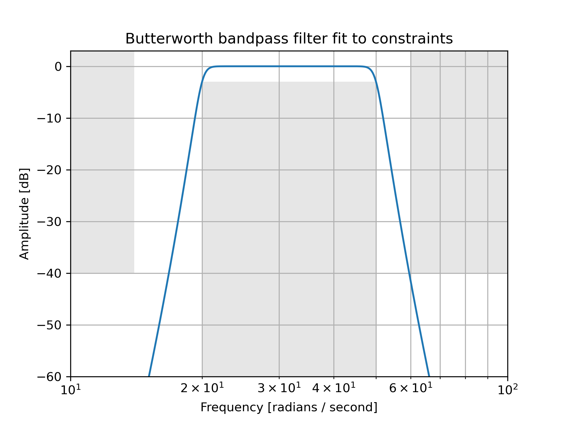
Design an analog bandpass filter with passband within 3 dB from 20 to 50 rad/s, while rejecting at least -40 dB below 14 and above 60 rad/s. Plot its frequency response, showing the passband and stopband constraints in gray.
>>> from scipy import signal
... import matplotlib.pyplot as plt
>>> N, Wn = signal.buttord([20, 50], [14, 60], 3, 40, True)
... b, a = signal.butter(N, Wn, 'band', True)
... w, h = signal.freqs(b, a, np.logspace(1, 2, 500))
... plt.semilogx(w, 20 * np.log10(abs(h)))
... plt.title('Butterworth bandpass filter fit to constraints')
... plt.xlabel('Frequency [radians / second]')
... plt.ylabel('Amplitude [dB]')
... plt.grid(which='both', axis='both')
... plt.fill([1,  14,  14,   1], [-40, -40, 99, 99], '0.9', lw=0) # stop
... plt.fill([20, 20,  50,  50], [-99, -3, -3, -99], '0.9', lw=0) # pass
... plt.fill([60, 60, 1e9, 1e9], [99, -40, -40, 99], '0.9', lw=0) # stop
... plt.axis([10, 100, -60, 3])
... plt.show()
The following pages refer to to this document either explicitly or contain code examples using this.
scipy.signal._filter_design.butter
scipy.signal._filter_design.ellipord
scipy.signal._filter_design.iirfilter
scipy.signal._filter_design.cheb1ord
scipy.signal._filter_design.buttord
scipy.signal._filter_design.cheb2ord
scipy.signal._filter_design.iirdesign
Hover to see nodes names; edges to Self not shown, Caped at 50 nodes.
Using a canvas is more power efficient and can get hundred of nodes ; but does not allow hyperlinks; , arrows or text (beyond on hover)
SVG is more flexible but power hungry; and does not scale well to 50 + nodes.
All aboves nodes referred to, (or are referred from) current nodes; Edges from Self to other have been omitted (or all nodes would be connected to the central node "self" which is not useful). Nodes are colored by the library they belong to, and scaled with the number of references pointing them