cont2discrete(system, dt, method='zoh', alpha=None)
By default, the routine uses a Zero-Order Hold (zoh) method to perform the transformation. Alternatively, a generalized bilinear transformation may be used, which includes the common Tustin's bilinear approximation, an Euler's method technique, or a backwards differencing technique.
The Zero-Order Hold (zoh) method is based on , the generalized bilinear approximation is based on and , the First-Order Hold (foh) method is based on .
The following gives the number of elements in the tuple and the interpretation:
1: (instance of
lti)2: (num, den)
3: (zeros, poles, gain)
4: (A, B, C, D)
The discretization time step.
Which method to use:
gbt: generalized bilinear transformation
bilinear: Tustin's approximation ("gbt" with alpha=0.5)
euler: Euler (or forward differencing) method ("gbt" with alpha=0)
backward_diff: Backwards differencing ("gbt" with alpha=1.0)
zoh: zero-order hold (default)
foh: first-order hold (versionadded: 1.3.0)
impulse: equivalent impulse response (versionadded: 1.3.0)
The generalized bilinear transformation weighting parameter, which should only be specified with method="gbt", and is ignored otherwise
Based on the input type, the output will be of the form
(num, den, dt) for transfer function input
(zeros, poles, gain, dt) for zeros-poles-gain input
(A, B, C, D, dt) for state-space system input
Transform a continuous to a discrete state-space system.
We can transform a continuous state-space system to a discrete one:
>>> import matplotlib.pyplot as plt
... from scipy.signal import cont2discrete, lti, dlti, dstep
Define a continuous state-space system.
>>> A = np.array([[0, 1],[-10., -3]])
... B = np.array([[0],[10.]])
... C = np.array([[1., 0]])
... D = np.array([[0.]])
... l_system = lti(A, B, C, D)
... t, x = l_system.step(T=np.linspace(0, 5, 100))
... fig, ax = plt.subplots()
... ax.plot(t, x, label='Continuous', linewidth=3)
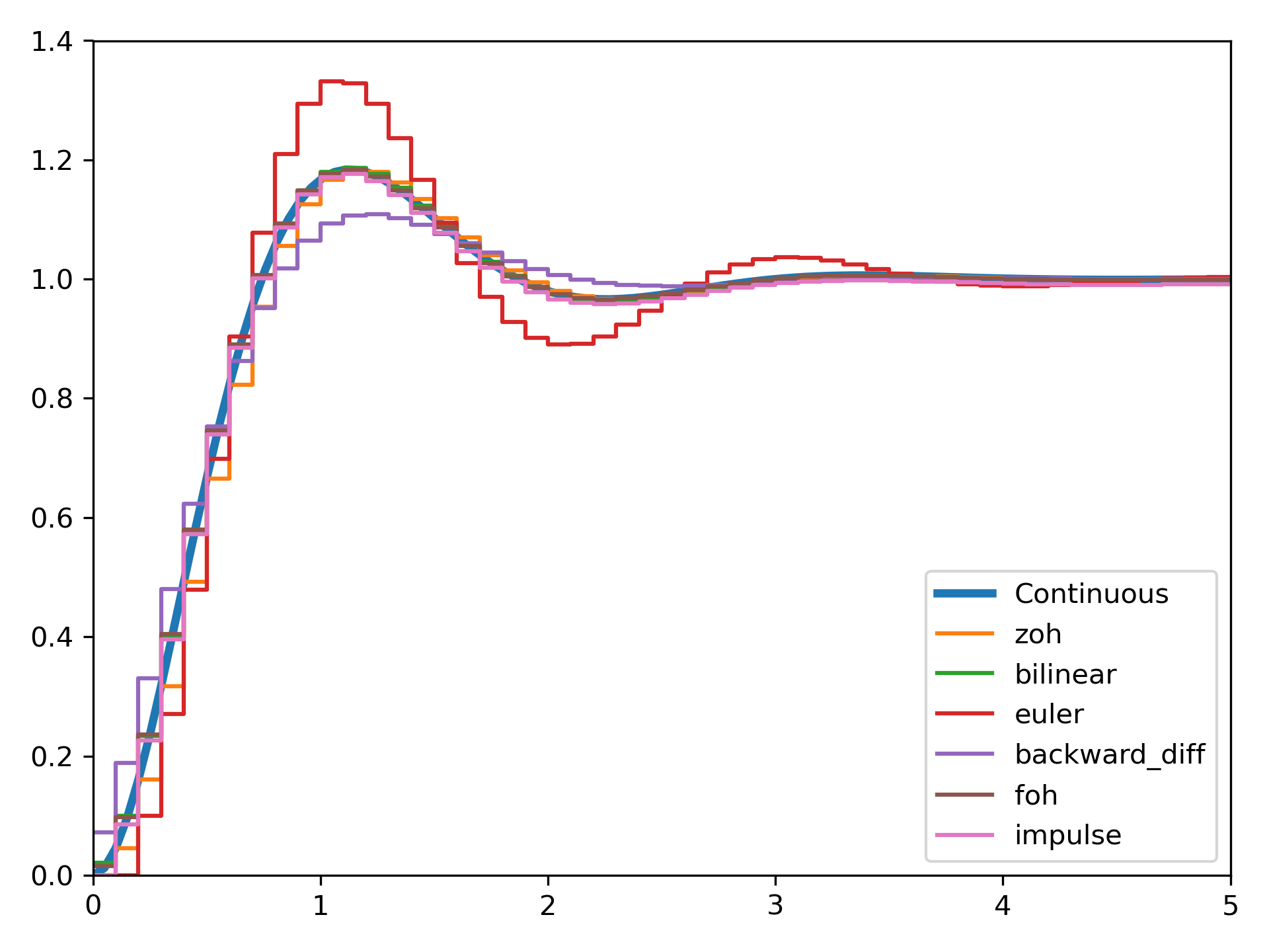
Transform it to a discrete state-space system using several methods.
>>> dt = 0.1
... for method in ['zoh', 'bilinear', 'euler', 'backward_diff', 'foh', 'impulse']:
...    d_system = cont2discrete((A, B, C, D), dt, method=method)
...    s, x_d = dstep(d_system)
...    ax.step(s, np.squeeze(x_d), label=method, where='post')
... ax.axis([t[0], t[-1], x[0], 1.4])
... ax.legend(loc='best')
... fig.tight_layout()
... plt.show()
The following pages refer to to this document either explicitly or contain code examples using this.
scipy.signal._ltisys.StateSpaceContinuous.to_discrete
scipy.signal._ltisys.dstep
scipy.signal._ltisys.ZerosPolesGainContinuous.to_discrete
scipy.signal._ltisys.lti.to_discrete
scipy.signal._ltisys.TransferFunctionContinuous.to_discrete
scipy.signal._ltisys.dimpulse
scipy.signal._lti_conversion.cont2discrete
scipy.signal._ltisys.dlsim
Hover to see nodes names; edges to Self not shown, Caped at 50 nodes.
Using a canvas is more power efficient and can get hundred of nodes ; but does not allow hyperlinks; , arrows or text (beyond on hover)
SVG is more flexible but power hungry; and does not scale well to 50 + nodes.
All aboves nodes referred to, (or are referred from) current nodes; Edges from Self to other have been omitted (or all nodes would be connected to the central node "self" which is not useful). Nodes are colored by the library they belong to, and scaled with the number of references pointing them