Determines a smoothing bicubic spline according to a given set of knots in the :None:None:`theta` and :None:None:`phi` directions.

Notes

For more information, see the :None:None:`FITPACK_` site about this function.

            <Unimplemented 'target' '.. _FITPACK: http://www.netlib.org/dierckx/sphere.f'>
           

Parameters

theta, phi, r : array_like

1-D sequences of data points (order is not important). Coordinates must be given in radians. Theta must lie within the interval [0, pi] , and phi must lie within the interval [0, 2pi] .

tt, tp : array_like

Strictly ordered 1-D sequences of knots coordinates. Coordinates must satisfy 0 < tt[i] < pi , 0 < tp[i] < 2*pi .

w : array_like, optional

Positive 1-D sequence of weights, of the same length as :None:None:`theta`, :None:None:`phi` and r.

eps : float, optional

A threshold for determining the effective rank of an over-determined linear system of equations. :None:None:`eps` should have a value within the open interval (0, 1) , the default is 1e-16.

Weighted least-squares bivariate spline approximation in spherical coordinates.

See Also

BivariateSpline

a base class for bivariate splines.

LSQBivariateSpline

a bivariate spline using weighted least-squares fitting

RectBivariateSpline

a bivariate spline over a rectangular mesh.

RectSphereBivariateSpline

a bivariate spline over a rectangular mesh on a sphere

SmoothBivariateSpline

a smoothing bivariate spline through the given points

SmoothSphereBivariateSpline

a smoothing bivariate spline in spherical coordinates

UnivariateSpline

a smooth univariate spline to fit a given set of data points.

bisplev

a function to evaluate a bivariate B-spline and its derivatives

bisplrep

a function to find a bivariate B-spline representation of a surface

Examples

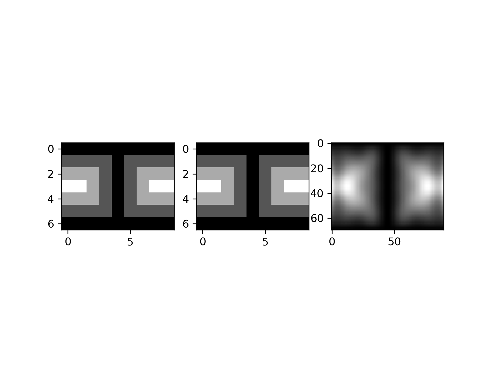
Suppose we have global data on a coarse grid (the input data does not have to be on a grid):

>>> from scipy.interpolate import LSQSphereBivariateSpline
... import matplotlib.pyplot as plt

>>> theta = np.linspace(0, np.pi, num=7)
... phi = np.linspace(0, 2*np.pi, num=9)
... data = np.empty((theta.shape[0], phi.shape[0]))
... data[:,0], data[0,:], data[-1,:] = 0., 0., 0.
... data[1:-1,1], data[1:-1,-1] = 1., 1.
... data[1,1:-1], data[-2,1:-1] = 1., 1.
... data[2:-2,2], data[2:-2,-2] = 2., 2.
... data[2,2:-2], data[-3,2:-2] = 2., 2.
... data[3,3:-2] = 3.
... data = np.roll(data, 4, 1)

We need to set up the interpolator object. Here, we must also specify the coordinates of the knots to use.

>>> lats, lons = np.meshgrid(theta, phi)
... knotst, knotsp = theta.copy(), phi.copy()
... knotst[0] += .0001
... knotst[-1] -= .0001
... knotsp[0] += .0001
... knotsp[-1] -= .0001
... lut = LSQSphereBivariateSpline(lats.ravel(), lons.ravel(),
...                                data.T.ravel(), knotst, knotsp)

As a first test, we'll see what the algorithm returns when run on the input coordinates

>>> data_orig = lut(theta, phi)

Finally we interpolate the data to a finer grid

>>> fine_lats = np.linspace(0., np.pi, 70)
... fine_lons = np.linspace(0., 2*np.pi, 90)
... data_lsq = lut(fine_lats, fine_lons)

>>> fig = plt.figure()
... ax1 = fig.add_subplot(131)
... ax1.imshow(data, interpolation='nearest')
... ax2 = fig.add_subplot(132)
... ax2.imshow(data_orig, interpolation='nearest')
... ax3 = fig.add_subplot(133)
... ax3.imshow(data_lsq, interpolation='nearest')
... plt.show()

See :

Back References

The following pages refer to to this document either explicitly or contain code examples using this.

scipy.interpolate._fitpack2.RectSphereBivariateSpline scipy.interpolate._fitpack2.SmoothBivariateSpline scipy.interpolate._fitpack2.BivariateSpline scipy.interpolate._fitpack2.LSQSphereBivariateSpline scipy.interpolate._fitpack2.RectBivariateSpline scipy.interpolate._fitpack2.LSQBivariateSpline scipy.interpolate._fitpack2.SmoothSphereBivariateSpline scipy.interpolate._fitpack2.UnivariateSpline

Local connectivity graph

Hover to see nodes names; edges to Self not shown, Caped at 50 nodes.

Using a canvas is more power efficient and can get hundred of nodes ; but does not allow hyperlinks; , arrows or text (beyond on hover)

SVG is more flexible but power hungry; and does not scale well to 50 + nodes.

All aboves nodes referred to, (or are referred from) current nodes; Edges from Self to other have been omitted (or all nodes would be connected to the central node "self" which is not useful). Nodes are colored by the library they belong to, and scaled with the number of references pointing them

---

GitHub : /scipy/interpolate/_fitpack2.py#1607
type: <class 'type'>
Commit: