Breakpoints. The same x
which was passed to the constructor.
Coefficients of the polynomials on each segment. The trailing dimensions match the dimensions of y, excluding axis
. For example, if y is 1-d, then c[k, i]
is a coefficient for (x-x[i])**(3-k)
on the segment between x[i]
and x[i+1]
.
Interpolation axis. The same axis which was passed to the constructor.
Interpolate data with a piecewise cubic polynomial which is twice continuously differentiable . The result is represented as a PPoly
instance with breakpoints matching the given data.
Parameters :None:None:`bc_type` and interpolate
work independently, i.e. the former controls only construction of a spline, and the latter only evaluation.
When a boundary condition is 'not-a-knot' and n = 2, it is replaced by a condition that the first derivative is equal to the linear interpolant slope. When both boundary conditions are 'not-a-knot' and n = 3, the solution is sought as a parabola passing through given points.
When 'not-a-knot' boundary conditions is applied to both ends, the resulting spline will be the same as returned by :None:None:`splrep` (with s=0
) and InterpolatedUnivariateSpline
, but these two methods use a representation in B-spline basis.
1-D array containing values of the independent variable. Values must be real, finite and in strictly increasing order.
Array containing values of the dependent variable. It can have arbitrary number of dimensions, but the length along axis
(see below) must match the length of x
. Values must be finite.
Axis along which y is assumed to be varying. Meaning that for x[i]
the corresponding values are np.take(y, i, axis=axis)
. Default is 0.
Boundary condition type. Two additional equations, given by the boundary conditions, are required to determine all coefficients of polynomials on each segment .
If :None:None:`bc_type` is a string, then the specified condition will be applied at both ends of a spline. Available conditions are:
'not-a-knot' (default): The first and second segment at a curve end are the same polynomial. It is a good default when there is no information on boundary conditions.
'periodic': The interpolated functions is assumed to be periodic of period x[-1] - x[0]
. The first and last value of y must be identical: y[0] == y[-1]
. This boundary condition will result in y'[0] == y'[-1]
and y''[0] == y''[-1]
.
'clamped': The first derivative at curves ends are zero. Assuming a 1D y, bc_type=((1, 0.0), (1, 0.0))
is the same condition.
'natural': The second derivative at curve ends are zero. Assuming a 1D y, bc_type=((2, 0.0), (2, 0.0))
is the same condition.
If :None:None:`bc_type` is a 2-tuple, the first and the second value will be applied at the curve start and end respectively. The tuple values can be one of the previously mentioned strings (except 'periodic') or a tuple :None:None:`(order, deriv_values)` allowing to specify arbitrary derivatives at curve ends:
:None:None:`order`: the derivative order, 1 or 2.
:None:None:`deriv_value`: array_like containing derivative values, shape must be the same as y, excluding axis
dimension. For example, if y is 1-D, then :None:None:`deriv_value` must be a scalar. If y is 3-D with the shape (n0, n1, n2) and axis=2, then :None:None:`deriv_value` must be 2-D and have the shape (n0, n1).
If bool, determines whether to extrapolate to out-of-bounds points based on first and last intervals, or to return NaNs. If 'periodic', periodic extrapolation is used. If None (default), extrapolate
is set to 'periodic' for bc_type='periodic'
and to True otherwise.
Cubic spline data interpolator.
Akima1DInterpolator
Akima 1D interpolator.
PPoly
Piecewise polynomial in terms of coefficients and breakpoints.
PchipInterpolator
PCHIP 1-D monotonic cubic interpolator.
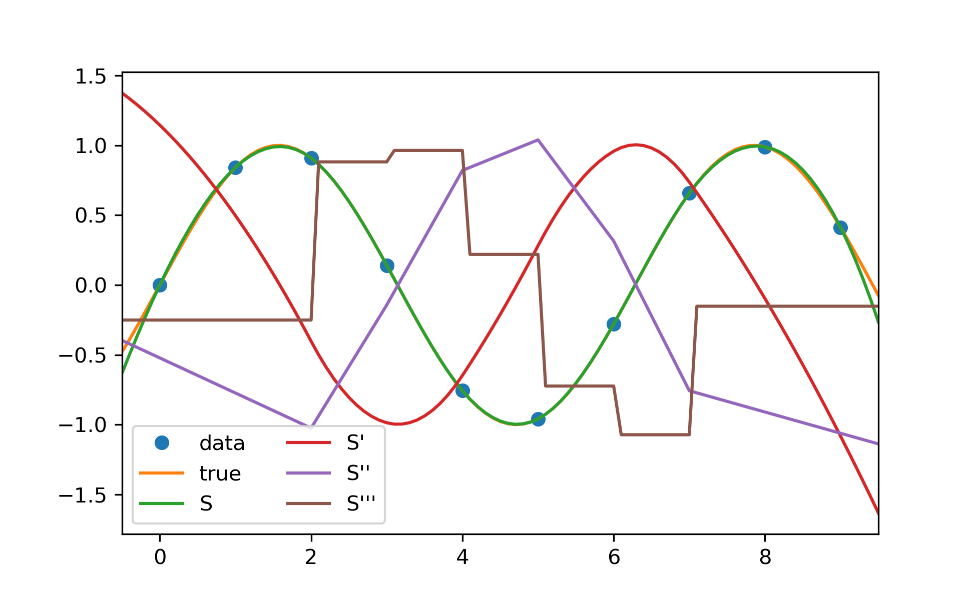
In this example the cubic spline is used to interpolate a sampled sinusoid. You can see that the spline continuity property holds for the first and second derivatives and violates only for the third derivative.
>>> from scipy.interpolate import CubicSpline
... import matplotlib.pyplot as plt
... x = np.arange(10)
... y = np.sin(x)
... cs = CubicSpline(x, y)
... xs = np.arange(-0.5, 9.6, 0.1)
... fig, ax = plt.subplots(figsize=(6.5, 4))
... ax.plot(x, y, 'o', label='data')
... ax.plot(xs, np.sin(xs), label='true')
... ax.plot(xs, cs(xs), label="S")
... ax.plot(xs, cs(xs, 1), label="S'")
... ax.plot(xs, cs(xs, 2), label="S''")
... ax.plot(xs, cs(xs, 3), label="S'''")
... ax.set_xlim(-0.5, 9.5)
... ax.legend(loc='lower left', ncol=2)
... plt.show()
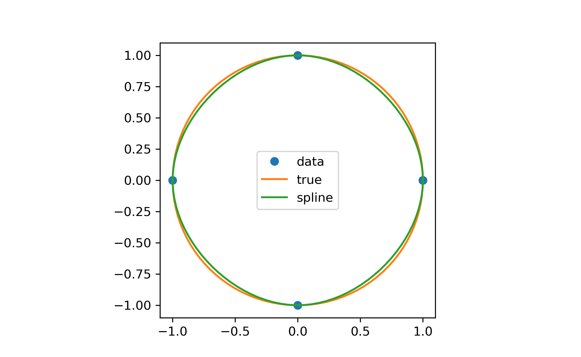
In the second example, the unit circle is interpolated with a spline. A periodic boundary condition is used. You can see that the first derivative values, ds/dx=0, ds/dy=1 at the periodic point (1, 0) are correctly computed. Note that a circle cannot be exactly represented by a cubic spline. To increase precision, more breakpoints would be required.
>>> theta = 2 * np.pi * np.linspace(0, 1, 5)
... y = np.c_[np.cos(theta), np.sin(theta)]
... cs = CubicSpline(theta, y, bc_type='periodic')
... print("ds/dx={:.1f} ds/dy={:.1f}".format(cs(0, 1)[0], cs(0, 1)[1]))
ds/dx=0.0 ds/dy=1.0
>>> xs = 2 * np.pi * np.linspace(0, 1, 100)
... fig, ax = plt.subplots(figsize=(6.5, 4))
... ax.plot(y[:, 0], y[:, 1], 'o', label='data')
... ax.plot(np.cos(xs), np.sin(xs), label='true')
... ax.plot(cs(xs)[:, 0], cs(xs)[:, 1], label='spline')
... ax.axes.set_aspect('equal')
... ax.legend(loc='center')
... plt.show()
The third example is the interpolation of a polynomial y = x**3 on the interval 0 <= x<= 1. A cubic spline can represent this function exactly. To achieve that we need to specify values and first derivatives at endpoints of the interval. Note that y' = 3 * x**2 and thus y'(0) = 0 and y'(1) = 3.
>>> cs = CubicSpline([0, 1], [0, 1], bc_type=((1, 0), (1, 3)))See :
... x = np.linspace(0, 1)
... np.allclose(x**3, cs(x)) True
The following pages refer to to this document either explicitly or contain code examples using this.
pandas.core.missing._cubicspline_interpolate
scipy.interpolate._cubic.CubicHermiteSpline
scipy.interpolate._cubic.CubicSpline
scipy.interpolate._cubic.Akima1DInterpolator
scipy.interpolate._cubic.PchipInterpolator
scipy.interpolate._bsplines.make_interp_spline
Hover to see nodes names; edges to Self not shown, Caped at 50 nodes.
Using a canvas is more power efficient and can get hundred of nodes ; but does not allow hyperlinks; , arrows or text (beyond on hover)
SVG is more flexible but power hungry; and does not scale well to 50 + nodes.
All aboves nodes referred to, (or are referred from) current nodes; Edges from Self to other have been omitted (or all nodes would be connected to the central node "self" which is not useful). Nodes are colored by the library they belong to, and scaled with the number of references pointing them