knot vector
spline coefficients
spline degree
If True, extrapolates the first and last polynomial pieces of b-spline functions active on the base interval.
Interpolation axis.
A read-only equivalent of (self.t, self.c, self.k)
where $B_{j, k; t}$
are B-spline basis functions of degree k and knots t.
B-spline basis elements are defined via
$$B_{i, 0}(x) = 1, \textrm{if $t_i \le x < t_{i+1}$, otherwise $0$,} B_{i, k}(x) = \frac{x - t_i}{t_{i+k} - t_i} B_{i, k-1}(x) + \frac{t_{i+k+1} - x}{t_{i+k+1} - t_{i+1}} B_{i+1, k-1}(x)$$Implementation details
At least k+1
coefficients are required for a spline of degree k, so that n >= k+1
. Additional coefficients, c[j]
with j > n
, are ignored.
B-spline basis elements of degree k form a partition of unity on the base interval, t[k] <= x <= t[n]
.
knots
spline coefficients
B-spline degree
whether to extrapolate beyond the base interval, t[k] .. t[n]
, or to return nans. If True, extrapolates the first and last polynomial pieces of b-spline functions active on the base interval. If 'periodic', periodic extrapolation is used. Default is True.
Interpolation axis. Default is zero.
Univariate spline in the B-spline basis.
Translating the recursive definition of B-splines into Python code, we have:
>>> def B(x, k, i, t):
...    if k == 0:
...       return 1.0 if t[i] <= x < t[i+1] else 0.0
...    if t[i+k] == t[i]:
...       c1 = 0.0
...    else:
...       c1 = (x - t[i])/(t[i+k] - t[i]) * B(x, k-1, i, t)
...    if t[i+k+1] == t[i+1]:
...       c2 = 0.0
...    else:
...       c2 = (t[i+k+1] - x)/(t[i+k+1] - t[i+1]) * B(x, k-1, i+1, t)
...    return c1 + c2
>>> def bspline(x, t, c, k):
...    n = len(t) - k - 1
...    assert (n >= k+1) and (len(c) >= n)
...    return sum(c[i] * B(x, k, i, t) for i in range(n))
Note that this is an inefficient (if straightforward) way to evaluate B-splines --- this spline class does it in an equivalent, but much more efficient way.
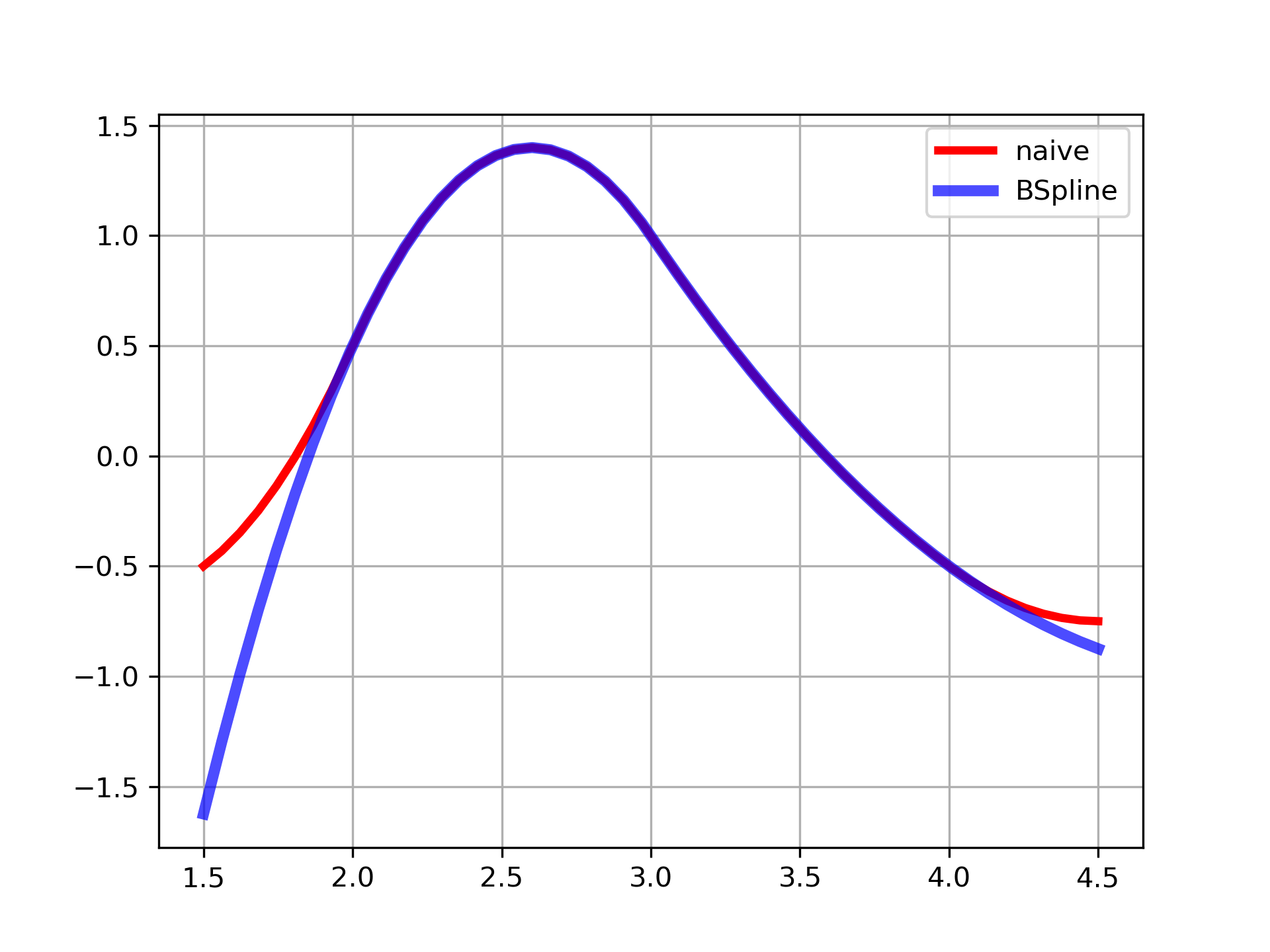
Here we construct a quadratic spline function on the base interval 2 <= x <= 4
and compare with the naive way of evaluating the spline:
>>> from scipy.interpolate import BSpline
... k = 2
... t = [0, 1, 2, 3, 4, 5, 6]
... c = [-1, 2, 0, -1]
... spl = BSpline(t, c, k)
... spl(2.5)
array(1.375)
>>> bspline(2.5, t, c, k)
1.375
Note that outside of the base interval results differ. This is because BSpline
extrapolates the first and last polynomial pieces of B-spline functions active on the base interval.
>>> import matplotlib.pyplot as plt
... fig, ax = plt.subplots()
... xx = np.linspace(1.5, 4.5, 50)
... ax.plot(xx, [bspline(x, t, c ,k) for x in xx], 'r-', lw=3, label='naive')
... ax.plot(xx, spl(xx), 'b-', lw=4, alpha=0.7, label='BSpline')
... ax.grid(True)
... ax.legend(loc='best')
... plt.show()

The following pages refer to to this document either explicitly or contain code examples using this.
scipy.interpolate._bsplines.BSpline.integrate
scipy.interpolate._bsplines.BSpline
scipy.interpolate._fitpack_py.insert
scipy.interpolate._bsplines.make_lsq_spline
scipy.interpolate._fitpack_py.splder
scipy.interpolate._fitpack_py.splrep
scipy.interpolate._fitpack_py.splantider
scipy.interpolate._fitpack_py.splev
scipy.interpolate._fitpack_py.sproot
scipy.interpolate._fitpack_py.splint
scipy.interpolate._bsplines.make_interp_spline
Hover to see nodes names; edges to Self not shown, Caped at 50 nodes.
Using a canvas is more power efficient and can get hundred of nodes ; but does not allow hyperlinks; , arrows or text (beyond on hover)
SVG is more flexible but power hungry; and does not scale well to 50 + nodes.
All aboves nodes referred to, (or are referred from) current nodes; Edges from Self to other have been omitted (or all nodes would be connected to the central node "self" which is not useful). Nodes are colored by the library they belong to, and scaled with the number of references pointing them