Document

scipy 1.8.0 Pypi GitHub Homepage

Other Docs

Notes Parameters Returns BackRef

make_lsq_spline(x, y, t, k=3, w=None, axis=0, check_finite=True)

The result is a linear combination

$$S(x) = \sum_j c_j B_j(x; t)$$

of the B-spline basis elements, $B_j(x; t)$ , which minimizes

$$\sum_{j} \left( w_j \times (S(x_j) - y_j) \right)^2$$

Notes

The number of data points must be larger than the spline degree k.

Knots t must satisfy the Schoenberg-Whitney conditions, i.e., there must be a subset of data points x[j] such that t[j] < x[j] < t[j+k+1] , for j=0, 1,...,n-k-2 .

Parameters

x : array_like, shape (m,): Abscissas.
y : array_like, shape (m, ...): Ordinates.
t : array_like, shape (n + k + 1,).: Knots. Knots and data points must satisfy Schoenberg-Whitney conditions.
k : int, optional: B-spline degree. Default is cubic, k=3.
w : array_like, shape (n,), optional: Weights for spline fitting. Must be positive. If None , then weights are all equal. Default is None .
axis : int, optional: Interpolation axis. Default is zero.
check_finite : bool, optional: Whether to check that the input arrays contain only finite numbers. Disabling may give a performance gain, but may result in problems (crashes, non-termination) if the inputs do contain infinities or NaNs. Default is True.

Returns

b : a BSpline object of the degree `k` with knots `t`.

Compute the (coefficients of) an LSQ B-spline.

Examples

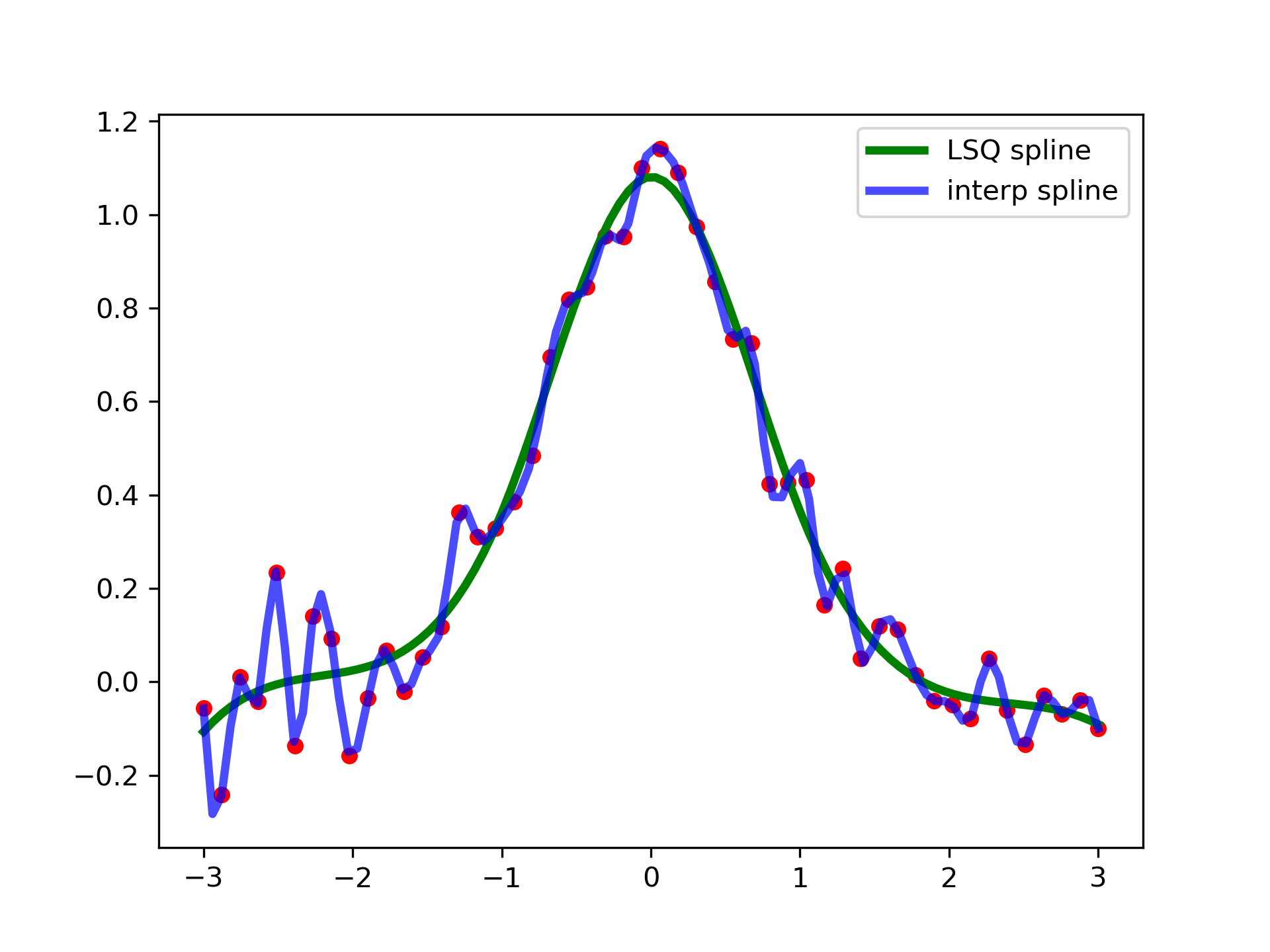
Generate some noisy data:

>>> rng = np.random.default_rng()
... x = np.linspace(-3, 3, 50)
... y = np.exp(-x**2) + 0.1 * rng.standard_normal(50)

Now fit a smoothing cubic spline with a pre-defined internal knots. Here we make the knot vector (k+1)-regular by adding boundary knots:

>>> from scipy.interpolate import make_lsq_spline, BSpline
... t = [-1, 0, 1]
... k = 3
... t = np.r_[(x[0],)*(k+1),
...           t,
...           (x[-1],)*(k+1)]
... spl = make_lsq_spline(x, y, t, k)

For comparison, we also construct an interpolating spline for the same set of data:

>>> from scipy.interpolate import make_interp_spline
... spl_i = make_interp_spline(x, y)

Plot both:

>>> import matplotlib.pyplot as plt
... xs = np.linspace(-3, 3, 100)
... plt.plot(x, y, 'ro', ms=5)
... plt.plot(xs, spl(xs), 'g-', lw=3, label='LSQ spline')
... plt.plot(xs, spl_i(xs), 'b-', lw=3, alpha=0.7, label='interp spline')
... plt.legend(loc='best')
... plt.show()

NaN handling: If the input arrays contain nan values, the result is not useful since the underlying spline fitting routines cannot deal with nan . A workaround is to use zero weights for not-a-number data points:

>>> y[8] = np.nan
... w = np.isnan(y)
... y[w] = 0.
... tck = make_lsq_spline(x, y, t, w=~w)

Notice the need to replace a nan by a numerical value (precise value does not matter as long as the corresponding weight is zero.)

See :

Back References

The following pages refer to to this document either explicitly or contain code examples using this.

scipy.interpolate._bsplines.make_lsq_spline scipy.interpolate._bsplines.make_interp_spline

Local connectivity graph

Hover to see nodes names; edges to Self not shown, Caped at 50 nodes.

Using a canvas is more power efficient and can get hundred of nodes ; but does not allow hyperlinks; , arrows or text (beyond on hover)

SVG is more flexible but power hungry; and does not scale well to 50 + nodes.

All aboves nodes referred to, (or are referred from) current nodes; Edges from Self to other have been omitted (or all nodes would be connected to the central node "self" which is not useful). Nodes are colored by the library they belong to, and scaled with the number of references pointing them