chirp(t, f0, t1, f1, method='linear', phi=0, vertex_zero=True)

In the following, 'Hz' should be interpreted as 'cycles per unit'; there is no requirement here that the unit is one second. The important distinction is that the units of rotation are cycles, not radians. Likewise, t could be a measurement of space instead of time.

Notes

There are four options for the method . The following formulas give the instantaneous frequency (in Hz) of the signal generated by :None:None:`chirp()`. For convenience, the shorter names shown below may also be used.

linear, lin, li:

f(t) = f0 + (f1 - f0) * t / t1

quadratic, quad, q:

The graph of the frequency f(t) is a parabola through (0, f0) and (t1, f1). By default, the vertex of the parabola is at (0, f0). If :None:None:`vertex_zero` is False, then the vertex is at (t1, f1). The formula is:

if vertex_zero is True:

f(t) = f0 + (f1 - f0) * t**2 / t1**2

else:

f(t) = f1 - (f1 - f0) * (t1 - t)**2 / t1**2

To use a more general quadratic function, or an arbitrary polynomial, use the function scipy.signal.sweep_poly .

logarithmic, log, lo:

f(t) = f0 * (f1/f0)**(t/t1)

f0 and f1 must be nonzero and have the same sign.

This signal is also known as a geometric or exponential chirp.

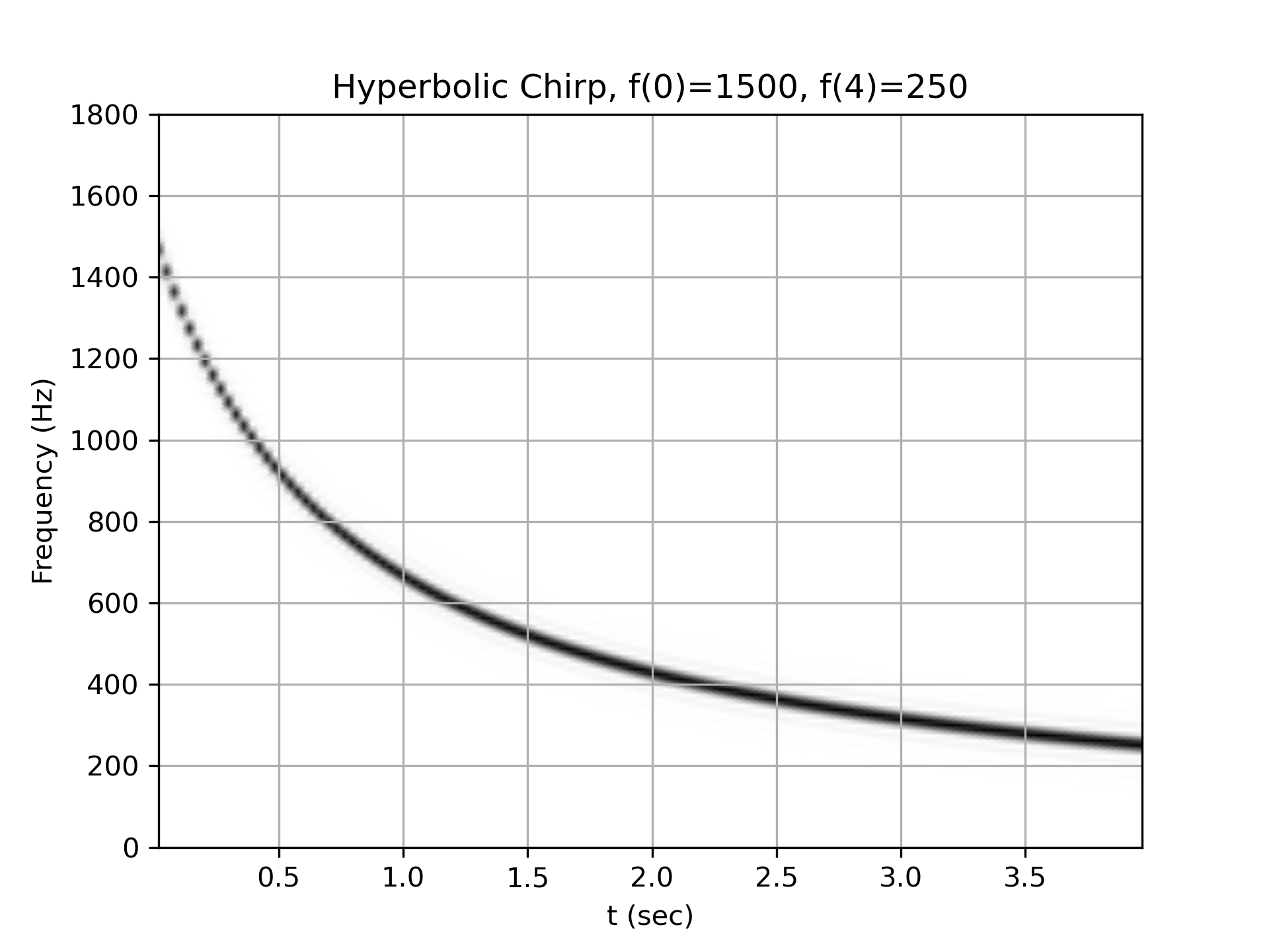
hyperbolic, hyp:

f(t) = f0*f1*t1 / ((f0 - f1)*t + f1*t1)

f0 and f1 must be nonzero.

Parameters

t : array_like

Times at which to evaluate the waveform.

f0 : float

Frequency (e.g. Hz) at time t=0.

t1 : float

Time at which :None:None:`f1` is specified.

f1 : float

Frequency (e.g. Hz) of the waveform at time :None:None:`t1`.

method : {'linear', 'quadratic', 'logarithmic', 'hyperbolic'}, optional

Kind of frequency sweep. If not given, :None:None:`linear` is assumed. See Notes below for more details.

phi : float, optional

Phase offset, in degrees. Default is 0.

vertex_zero : bool, optional

This parameter is only used when method is 'quadratic'. It determines whether the vertex of the parabola that is the graph of the frequency is at t=0 or t=t1.

Returns

y : ndarray

A numpy array containing the signal evaluated at t with the requested time-varying frequency. More precisely, the function returns cos(phase + (pi/180)*phi) where :None:None:`phase` is the integral (from 0 to t) of 2*pi*f(t) . f(t) is defined below.

Frequency-swept cosine generator.

See Also

sweep_poly

Examples

The following will be used in the examples:

>>> from scipy.signal import chirp, spectrogram
... import matplotlib.pyplot as plt

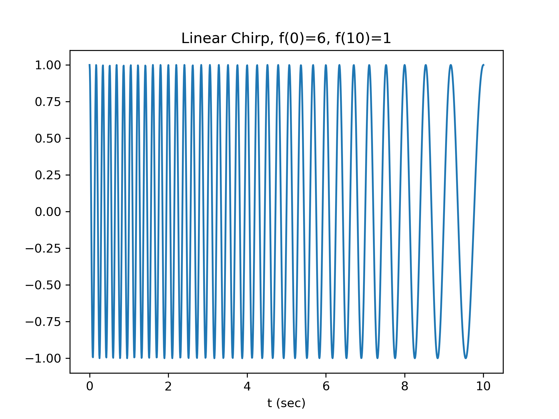
For the first example, we'll plot the waveform for a linear chirp from 6 Hz to 1 Hz over 10 seconds:

>>> t = np.linspace(0, 10, 1500)
... w = chirp(t, f0=6, f1=1, t1=10, method='linear')
... plt.plot(t, w)
... plt.title("Linear Chirp, f(0)=6, f(10)=1")
... plt.xlabel('t (sec)')
... plt.show()

For the remaining examples, we'll use higher frequency ranges, and demonstrate the result using scipy.signal.spectrogram . We'll use a 4 second interval sampled at 7200 Hz.

>>> fs = 7200
... T = 4
... t = np.arange(0, int(T*fs)) / fs

We'll use this function to plot the spectrogram in each example.

>>> def plot_spectrogram(title, w, fs):
...     ff, tt, Sxx = spectrogram(w, fs=fs, nperseg=256, nfft=576)
...     plt.pcolormesh(tt, ff[:145], Sxx[:145], cmap='gray_r', shading='gouraud')
...     plt.title(title)
...     plt.xlabel('t (sec)')
...     plt.ylabel('Frequency (Hz)')
...     plt.grid()
...

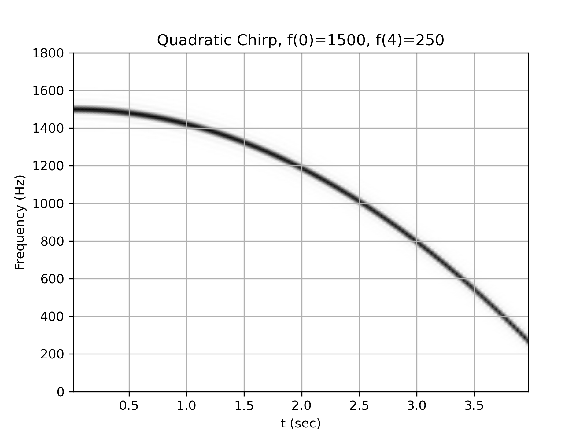
Quadratic chirp from 1500 Hz to 250 Hz (vertex of the parabolic curve of the frequency is at t=0):

>>> w = chirp(t, f0=1500, f1=250, t1=T, method='quadratic')
... plot_spectrogram(f'Quadratic Chirp, f(0)=1500, f({T})=250', w, fs)
... plt.show()

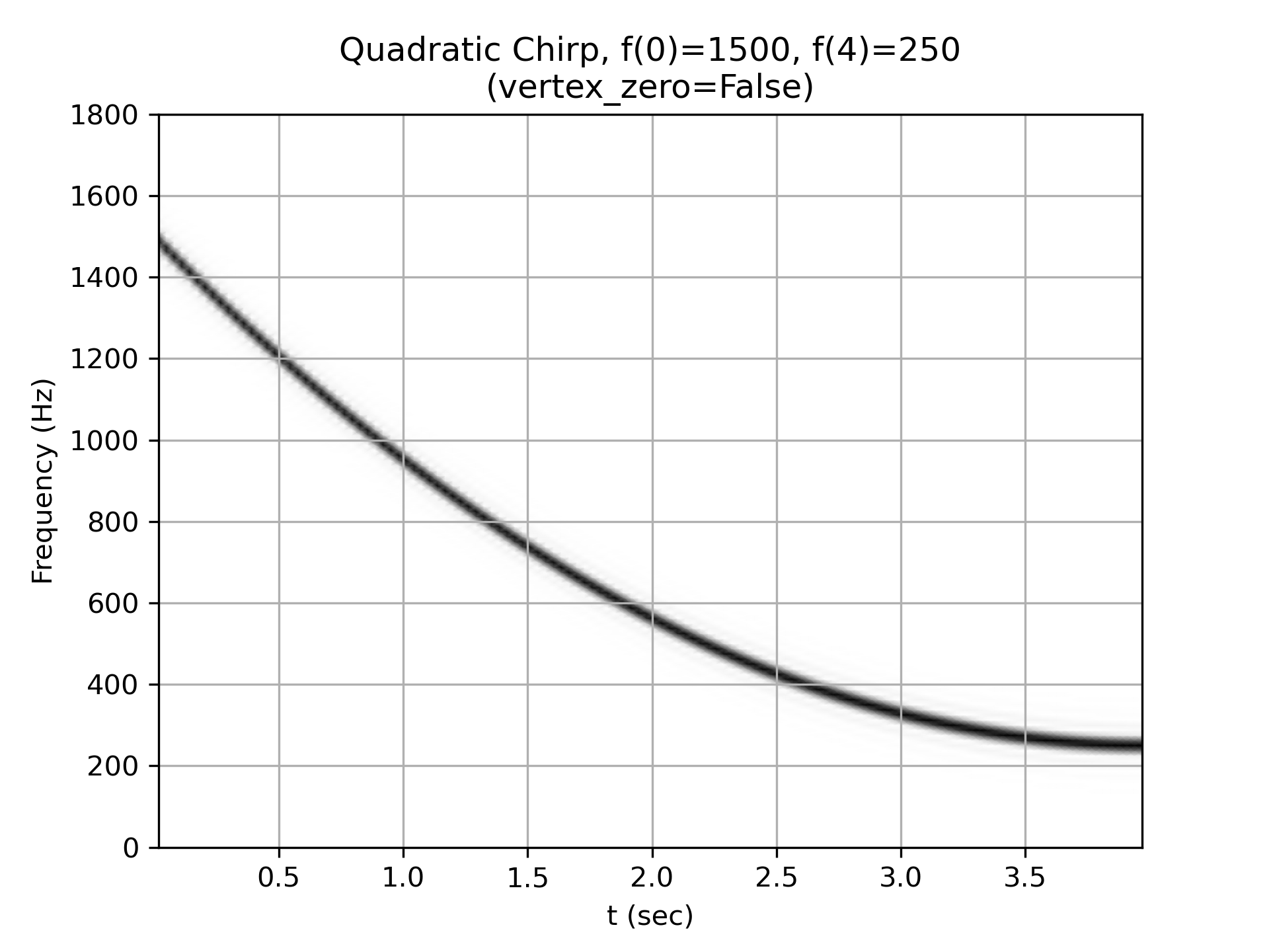
Quadratic chirp from 1500 Hz to 250 Hz (vertex of the parabolic curve of the frequency is at t=T):

>>> w = chirp(t, f0=1500, f1=250, t1=T, method='quadratic',
...           vertex_zero=False)
... plot_spectrogram(f'Quadratic Chirp, f(0)=1500, f({T})=250\n' +
...                  '(vertex_zero=False)', w, fs)
... plt.show()

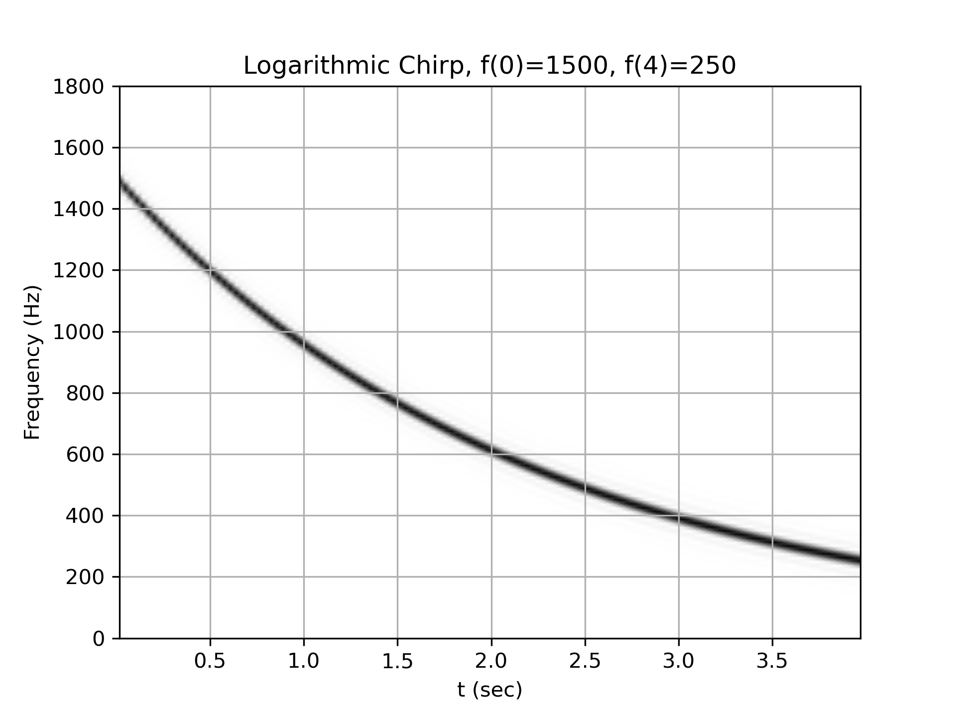
Logarithmic chirp from 1500 Hz to 250 Hz:

>>> w = chirp(t, f0=1500, f1=250, t1=T, method='logarithmic')
... plot_spectrogram(f'Logarithmic Chirp, f(0)=1500, f({T})=250', w, fs)
... plt.show()

Hyperbolic chirp from 1500 Hz to 250 Hz:

>>> w = chirp(t, f0=1500, f1=250, t1=T, method='hyperbolic')
... plot_spectrogram(f'Hyperbolic Chirp, f(0)=1500, f({T})=250', w, fs)
... plt.show()

See :

Back References

The following pages refer to to this document either explicitly or contain code examples using this.

scipy.signal._waveforms.chirp scipy.signal._waveforms._chirp_phase scipy.signal._waveforms.sweep_poly scipy.signal._signaltools.hilbert scipy.signal._peak_finding.peak_widths

Local connectivity graph

Hover to see nodes names; edges to Self not shown, Caped at 50 nodes.

Using a canvas is more power efficient and can get hundred of nodes ; but does not allow hyperlinks; , arrows or text (beyond on hover)

SVG is more flexible but power hungry; and does not scale well to 50 + nodes.

All aboves nodes referred to, (or are referred from) current nodes; Edges from Self to other have been omitted (or all nodes would be connected to the central node "self" which is not useful). Nodes are colored by the library they belong to, and scaled with the number of references pointing them

---

GitHub : /scipy/signal/_waveforms.py#261
type: <class 'function'>
Commit: