sweep_poly(t, poly, phi=0)
This function generates a sinusoidal function whose instantaneous frequency varies with time. The frequency at time t is given by the polynomial :None:None:`poly`.
If :None:None:`poly` is a list or ndarray of length :None:None:`n`, then the elements of :None:None:`poly` are the coefficients of the polynomial, and the instantaneous frequency is:
f(t) = poly[0]*t**(n-1) + poly[1]*t**(n-2) + ... + poly[n-1]
If :None:None:`poly` is an instance of numpy.poly1d
, then the instantaneous frequency is:
f(t) = poly(t)
Finally, the output s is:
cos(phase + (pi/180)*phi)
where :None:None:`phase` is the integral from 0 to t of 2 * pi * f(t)
, f(t)
as defined above.
Times at which to evaluate the waveform.
The desired frequency expressed as a polynomial. If :None:None:`poly` is a list or ndarray of length n, then the elements of :None:None:`poly` are the coefficients of the polynomial, and the instantaneous frequency is
f(t) = poly[0]*t**(n-1) + poly[1]*t**(n-2) + ... + poly[n-1]
If :None:None:`poly` is an instance of numpy.poly1d, then the instantaneous frequency is
f(t) = poly(t)
Phase offset, in degrees, Default: 0.
A numpy array containing the signal evaluated at t with the requested time-varying frequency. More precisely, the function returns cos(phase + (pi/180)*phi)
, where :None:None:`phase` is the integral (from 0 to t) of 2 * pi * f(t)
; f(t)
is defined above.
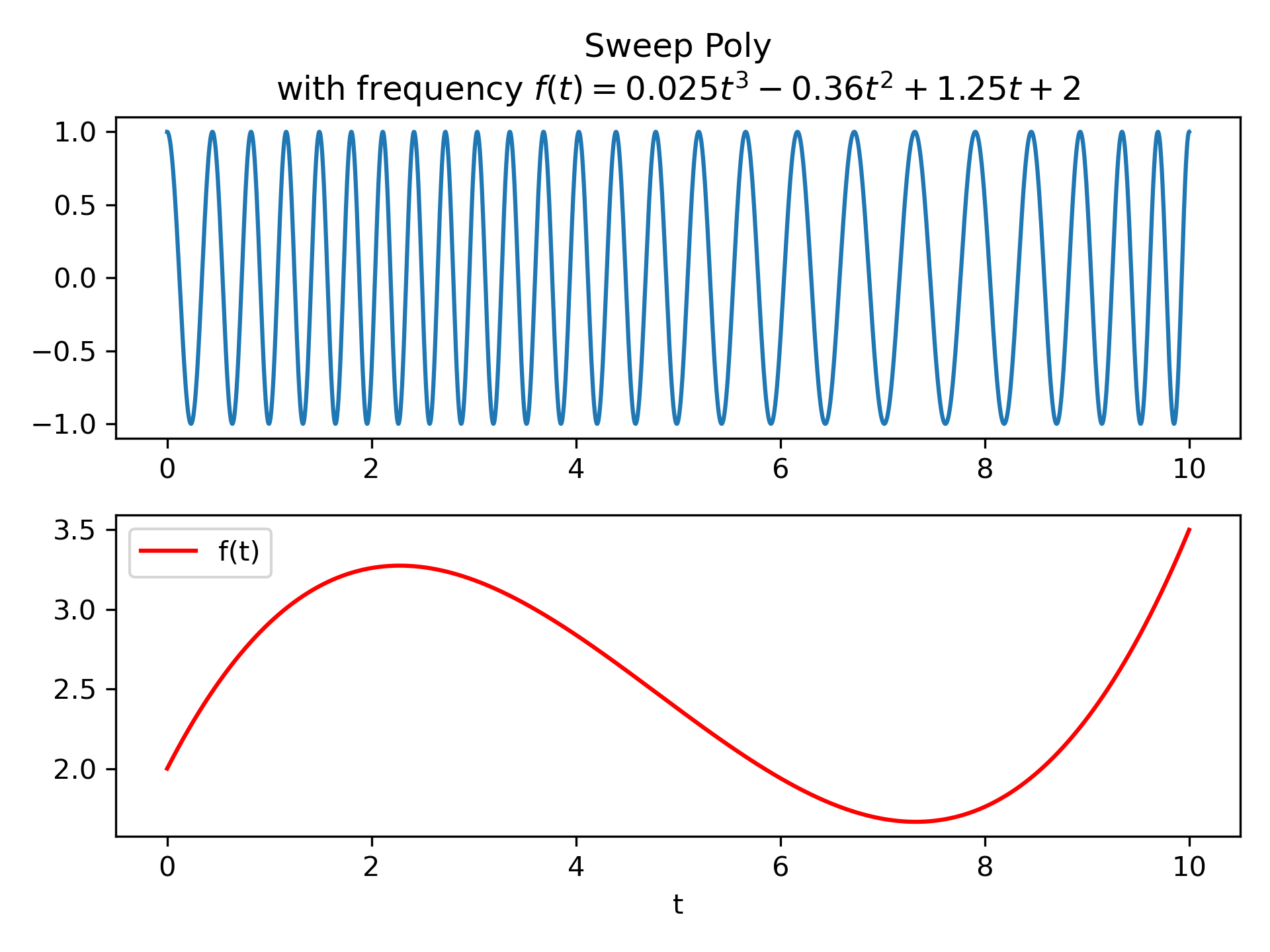
Frequency-swept cosine generator, with a time-dependent frequency.
f(t) = 0.025*t**3 - 0.36*t**2 + 1.25*t + 2
over the interval 0 <= t <= 10.
>>> from scipy.signal import sweep_poly
... p = np.poly1d([0.025, -0.36, 1.25, 2.0])
... t = np.linspace(0, 10, 5001)
... w = sweep_poly(t, p)
Plot it:
>>> import matplotlib.pyplot as plt
... plt.subplot(2, 1, 1)
... plt.plot(t, w)
... plt.title("Sweep Poly\nwith frequency " +
...           "$f(t) = 0.025t^3 - 0.36t^2 + 1.25t + 2$")
... plt.subplot(2, 1, 2)
... plt.plot(t, p(t), 'r', label='f(t)')
... plt.legend()
... plt.xlabel('t')
... plt.tight_layout()
... plt.show()
The following pages refer to to this document either explicitly or contain code examples using this.
scipy.signal._waveforms.sweep_poly
scipy.signal._waveforms._sweep_poly_phase
scipy.signal._waveforms.chirp
Hover to see nodes names; edges to Self not shown, Caped at 50 nodes.
Using a canvas is more power efficient and can get hundred of nodes ; but does not allow hyperlinks; , arrows or text (beyond on hover)
SVG is more flexible but power hungry; and does not scale well to 50 + nodes.
All aboves nodes referred to, (or are referred from) current nodes; Edges from Self to other have been omitted (or all nodes would be connected to the central node "self" which is not useful). Nodes are colored by the library they belong to, and scaled with the number of references pointing them