Can be used for smoothing data.
Currently, only the smoothing spline approximation ( iopt[0] = 0
and iopt[0] = 1
in the FITPACK routine) is supported. The exact least-squares spline approximation is not implemented yet.
When actually performing the interpolation, the requested v values must lie within the same length 2pi interval that the original v values were chosen from.
For more information, see the :None:None:`FITPACK_` site about this function.
<Unimplemented 'target' '.. _FITPACK: http://www.netlib.org/dierckx/spgrid.f'>
1-D array of colatitude coordinates in strictly ascending order. Coordinates must be given in radians and lie within the open interval (0, pi)
.
1-D array of longitude coordinates in strictly ascending order. Coordinates must be given in radians. First element ( v[0]
) must lie within the interval [-pi, pi)
. Last element ( v[-1]
) must satisfy v[-1] <= v[0] + 2*pi
.
2-D array of data with shape (u.size, v.size)
.
Positive smoothing factor defined for estimation condition ( s=0
is for interpolation).
Order of continuity at the poles u=0
( pole_continuity[0]
) and u=pi
( pole_continuity[1]
). The order of continuity at the pole will be 1 or 0 when this is True or False, respectively. Defaults to False.
Data values at the poles u=0
and u=pi
. Either the whole parameter or each individual element can be None. Defaults to None.
Data value exactness at the poles u=0
and u=pi
. If True, the value is considered to be the right function value, and it will be fitted exactly. If False, the value will be considered to be a data value just like the other data values. Defaults to False.
For the poles at u=0
and u=pi
, specify whether or not the approximation has vanishing derivatives. Defaults to False.
Bivariate spline approximation over a rectangular mesh on a sphere.
BivariateSpline
a base class for bivariate splines.
LSQBivariateSpline
a bivariate spline using weighted least-squares fitting
LSQSphereBivariateSpline
a bivariate spline in spherical coordinates using weighted least-squares fitting
RectBivariateSpline
a bivariate spline over a rectangular mesh.
SmoothBivariateSpline
a smoothing bivariate spline through the given points
SmoothSphereBivariateSpline
a smoothing bivariate spline in spherical coordinates
UnivariateSpline
a smooth univariate spline to fit a given set of data points.
bisplev
a function to evaluate a bivariate B-spline and its derivatives
bisplrep
a function to find a bivariate B-spline representation of a surface
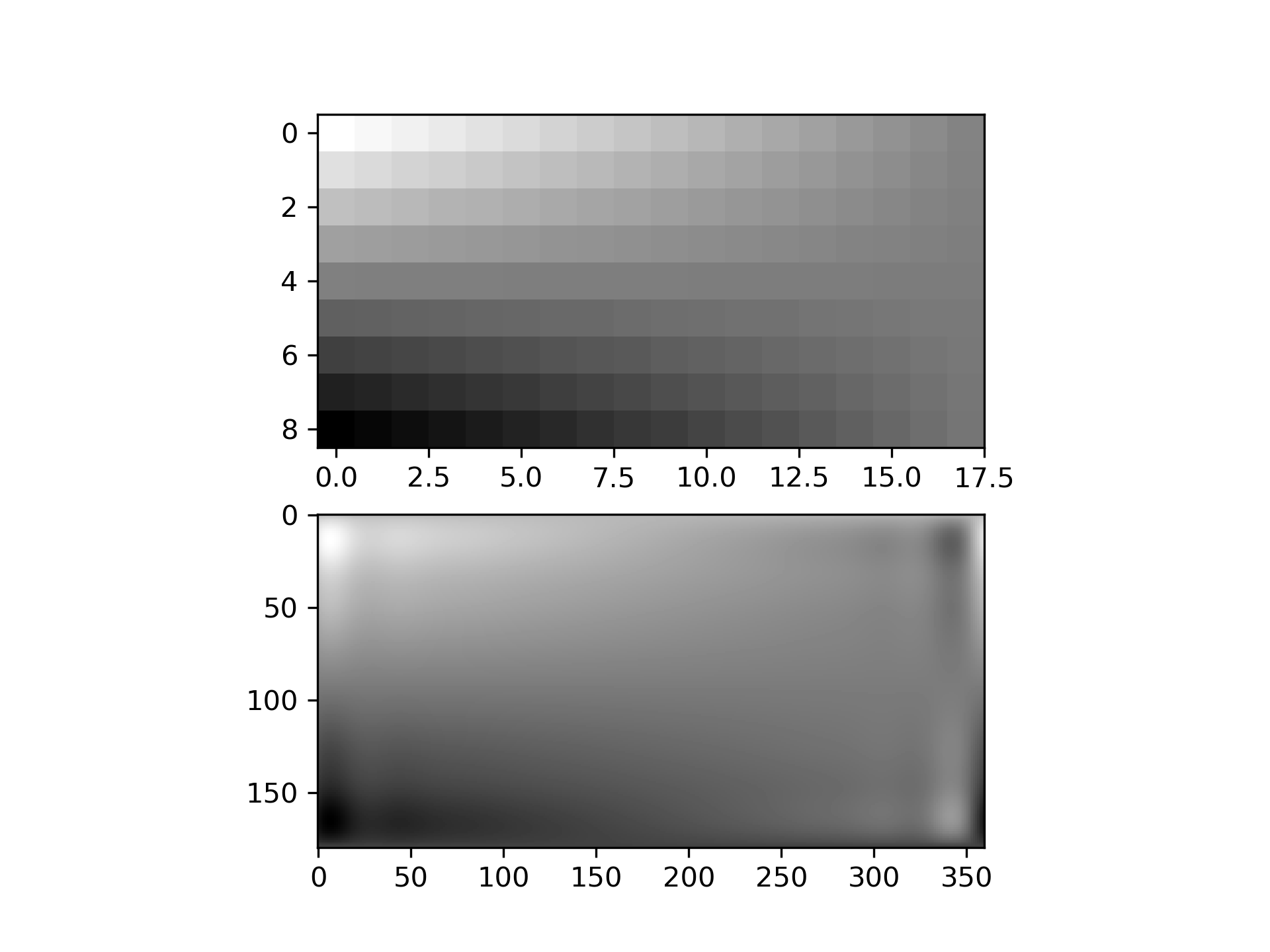
Suppose we have global data on a coarse grid
>>> lats = np.linspace(10, 170, 9) * np.pi / 180.
... lons = np.linspace(0, 350, 18) * np.pi / 180.
... data = np.dot(np.atleast_2d(90. - np.linspace(-80., 80., 18)).T,
...               np.atleast_2d(180. - np.abs(np.linspace(0., 350., 9)))).T
We want to interpolate it to a global one-degree grid
>>> new_lats = np.linspace(1, 180, 180) * np.pi / 180
... new_lons = np.linspace(1, 360, 360) * np.pi / 180
... new_lats, new_lons = np.meshgrid(new_lats, new_lons)
We need to set up the interpolator object
>>> from scipy.interpolate import RectSphereBivariateSpline
... lut = RectSphereBivariateSpline(lats, lons, data)
Finally we interpolate the data. The RectSphereBivariateSpline
object only takes 1-D arrays as input, therefore we need to do some reshaping.
>>> data_interp = lut.ev(new_lats.ravel(),
...                      new_lons.ravel()).reshape((360, 180)).T
Looking at the original and the interpolated data, one can see that the interpolant reproduces the original data very well:
>>> import matplotlib.pyplot as plt
... fig = plt.figure()
... ax1 = fig.add_subplot(211)
... ax1.imshow(data, interpolation='nearest')
... ax2 = fig.add_subplot(212)
... ax2.imshow(data_interp, interpolation='nearest')
... plt.show()
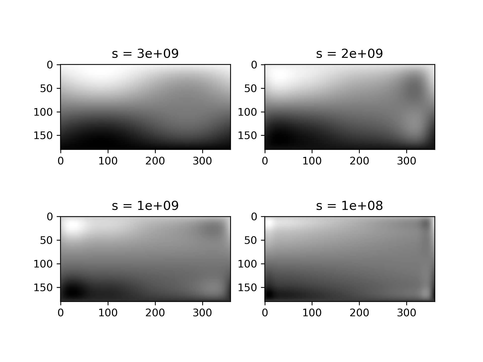
Choosing the optimal value of s
can be a delicate task. Recommended values for s
depend on the accuracy of the data values. If the user has an idea of the statistical errors on the data, she can also find a proper estimate for s
. By assuming that, if she specifies the right s
, the interpolator will use a spline f(u,v)
which exactly reproduces the function underlying the data, she can evaluate sum((r(i,j)-s(u(i),v(j)))**2)
to find a good estimate for this s
. For example, if she knows that the statistical errors on her r(i,j)
-values are not greater than 0.1, she may expect that a good s
should have a value not larger than u.size * v.size * (0.1)**2
.
If nothing is known about the statistical error in r(i,j)
, s
must be determined by trial and error. The best is then to start with a very large value of s
(to determine the least-squares polynomial and the corresponding upper bound fp0
for s
) and then to progressively decrease the value of s
(say by a factor 10 in the beginning, i.e. s = fp0 / 10, fp0 / 100, ...
and more carefully as the approximation shows more detail) to obtain closer fits.
The interpolation results for different values of s
give some insight into this process:
>>> fig2 = plt.figure()
... s = [3e9, 2e9, 1e9, 1e8]
... for idx, sval in enumerate(s, 1):
...     lut = RectSphereBivariateSpline(lats, lons, data, s=sval)
...     data_interp = lut.ev(new_lats.ravel(),
...                          new_lons.ravel()).reshape((360, 180)).T
...     ax = fig2.add_subplot(2, 2, idx)
...     ax.imshow(data_interp, interpolation='nearest')
...     ax.set_title(f"s = {sval:g}")
... plt.show()
The following pages refer to to this document either explicitly or contain code examples using this.
scipy.interpolate._fitpack2.RectSphereBivariateSpline
scipy.interpolate._fitpack2.SmoothBivariateSpline
scipy.interpolate._fitpack2.BivariateSpline
scipy.interpolate._fitpack2.LSQSphereBivariateSpline
scipy.interpolate._fitpack2.RectBivariateSpline
scipy.interpolate._fitpack2.LSQBivariateSpline
scipy.interpolate._fitpack2.SmoothSphereBivariateSpline
scipy.interpolate._fitpack2.UnivariateSpline
Hover to see nodes names; edges to Self not shown, Caped at 50 nodes.
Using a canvas is more power efficient and can get hundred of nodes ; but does not allow hyperlinks; , arrows or text (beyond on hover)
SVG is more flexible but power hungry; and does not scale well to 50 + nodes.
All aboves nodes referred to, (or are referred from) current nodes; Edges from Self to other have been omitted (or all nodes would be connected to the central node "self" which is not useful). Nodes are colored by the library they belong to, and scaled with the number of references pointing them