This is a specialization of the chirp z-transform (CZT
) for a set of equally-spaced frequencies around the unit circle, used to calculate a section of the FFT more efficiently than calculating the entire FFT and truncating.
The defaults are chosen such that f(x, 2)
is equivalent to fft.fft(x)
and, if m > len(x)
, that f(x, 2, m)
is equivalent to fft.fft(x, m)
.
Sampling frequency is 1/dt, the time step between samples in the signal :None:None:`x`. The unit circle corresponds to frequencies from 0 up to the sampling frequency. The default sampling frequency of 2 means that :None:None:`f1`, :None:None:`f2` values up to the Nyquist frequency are in the range [0, 1). For :None:None:`f1`, :None:None:`f2` values expressed in radians, a sampling frequency of 2*pi should be used.
Remember that a zoom FFT can only interpolate the points of the existing FFT. It cannot help to resolve two separate nearby frequencies. Frequency resolution can only be increased by increasing acquisition time.
These functions are implemented using Bluestein's algorithm (as is scipy.fft
).
The size of the signal.
A length-2 sequence [`f1`, :None:None:`f2`] giving the frequency range, or a scalar, for which the range [0, :None:None:`fn`] is assumed.
The number of points to evaluate. Default is n.
The sampling frequency. If fs=10
represented 10 kHz, for example, then :None:None:`f1` and :None:None:`f2` would also be given in kHz. The default sampling frequency is 2, so :None:None:`f1` and :None:None:`f2` should be in the range [0, 1] to keep the transform below the Nyquist frequency.
If True, :None:None:`f2` is the last sample. Otherwise, it is not included. Default is False.
Callable object f(x, axis=-1)
for computing the zoom FFT on :None:None:`x`.
Create a callable zoom FFT transform function.
zoom_fft
Convenience function for calculating a zoom FFT.
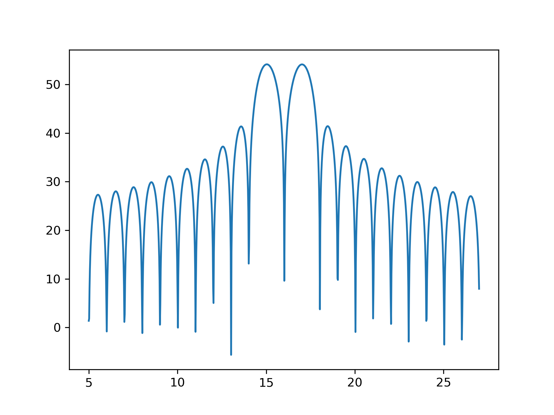
To plot the transform results use something like the following:
>>> from scipy.signal import ZoomFFT
... t = np.linspace(0, 1, 1021)
... x = np.cos(2*np.pi*15*t) + np.sin(2*np.pi*17*t)
... f1, f2 = 5, 27
... transform = ZoomFFT(len(x), [f1, f2], len(x), fs=1021)
... X = transform(x)
... f = np.linspace(f1, f2, len(x))
... import matplotlib.pyplot as plt
... plt.plot(f, 20*np.log10(np.abs(X)))
... plt.show()
The following pages refer to to this document either explicitly or contain code examples using this.
scipy.signal._czt.zoom_fft
scipy.signal._czt.ZoomFFT
Hover to see nodes names; edges to Self not shown, Caped at 50 nodes.
Using a canvas is more power efficient and can get hundred of nodes ; but does not allow hyperlinks; , arrows or text (beyond on hover)
SVG is more flexible but power hungry; and does not scale well to 50 + nodes.
All aboves nodes referred to, (or are referred from) current nodes; Edges from Self to other have been omitted (or all nodes would be connected to the central node "self" which is not useful). Nodes are colored by the library they belong to, and scaled with the number of references pointing them