barycentric_interpolate(xi, yi, x, axis=0)
Constructs a polynomial that passes through a given set of points, then evaluates the polynomial. For reasons of numerical stability, this function does not compute the coefficients of the polynomial.
This function uses a "barycentric interpolation" method that treats the problem as a special case of rational function interpolation. This algorithm is quite stable, numerically, but even in a world of exact computation, unless the x coordinates are chosen very carefully - Chebyshev zeros (e.g., cos(i*pi/n)) are a good choice - polynomial interpolation itself is a very ill-conditioned process due to the Runge phenomenon.
Construction of the interpolation weights is a relatively slow process. If you want to call this many times with the same xi (but possibly varying yi or x) you should use the class BarycentricInterpolator
. This is what this function uses internally.
1-D array of x coordinates of the points the polynomial should pass through
The y coordinates of the points the polynomial should pass through.
Points to evaluate the interpolator at.
Axis in the yi array corresponding to the x-coordinate values.
Interpolated values. Shape is determined by replacing the interpolation axis in the original array with the shape of x.
Convenience function for polynomial interpolation.
BarycentricInterpolator
Bary centric interpolator
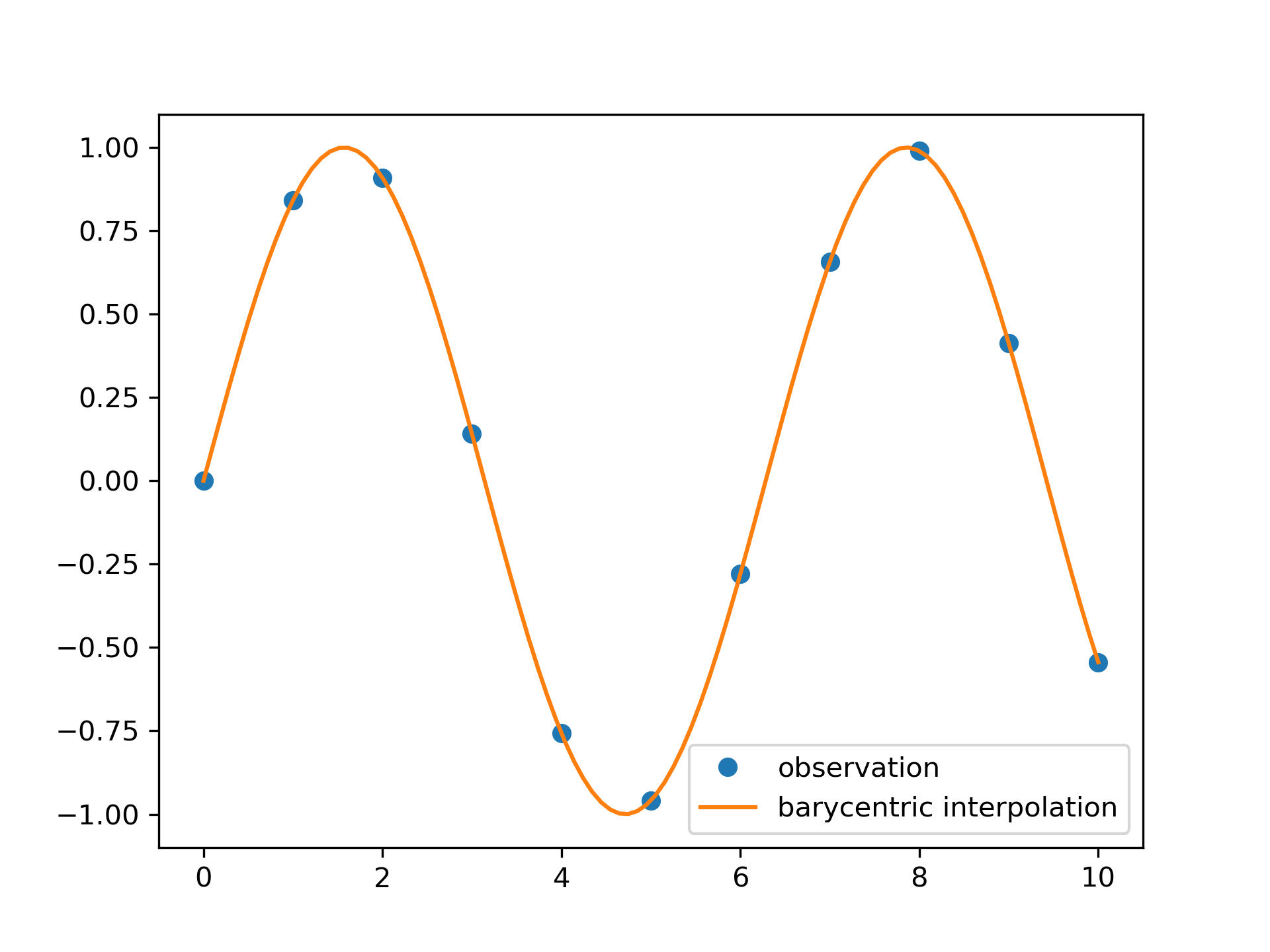
We can interpolate 2D observed data using barycentric interpolation:
>>> import matplotlib.pyplot as plt
... from scipy.interpolate import barycentric_interpolate
... x_observed = np.linspace(0.0, 10.0, 11)
... y_observed = np.sin(x_observed)
... x = np.linspace(min(x_observed), max(x_observed), num=100)
... y = barycentric_interpolate(x_observed, y_observed, x)
... plt.plot(x_observed, y_observed, "o", label="observation")
... plt.plot(x, y, label="barycentric interpolation")
... plt.legend()
... plt.show()
The following pages refer to to this document either explicitly or contain code examples using this.
scipy.interpolate._polyint.barycentric_interpolate
Hover to see nodes names; edges to Self not shown, Caped at 50 nodes.
Using a canvas is more power efficient and can get hundred of nodes ; but does not allow hyperlinks; , arrows or text (beyond on hover)
SVG is more flexible but power hungry; and does not scale well to 50 + nodes.
All aboves nodes referred to, (or are referred from) current nodes; Edges from Self to other have been omitted (or all nodes would be connected to the central node "self" which is not useful). Nodes are colored by the library they belong to, and scaled with the number of references pointing them