approximate_taylor_polynomial(f, x, degree, scale, order=None)
The appropriate choice of "scale" is a trade-off; too large and the function differs from its Taylor polynomial too much to get a good answer, too small and round-off errors overwhelm the higher-order terms. The algorithm used becomes numerically unstable around order 30 even under ideal circumstances.
Choosing order somewhat larger than degree may improve the higher-order terms.
The function whose Taylor polynomial is sought. Should accept a vector of x values.
The point at which the polynomial is to be evaluated.
The degree of the Taylor polynomial
The width of the interval to use to evaluate the Taylor polynomial. Function values spread over a range this wide are used to fit the polynomial. Must be chosen carefully.
The order of the polynomial to be used in the fitting; f will be evaluated order+1
times. If None, use degree
.
The Taylor polynomial (translated to the origin, so that for example p(0)=f(x)).
Estimate the Taylor polynomial of f at x by polynomial fitting.
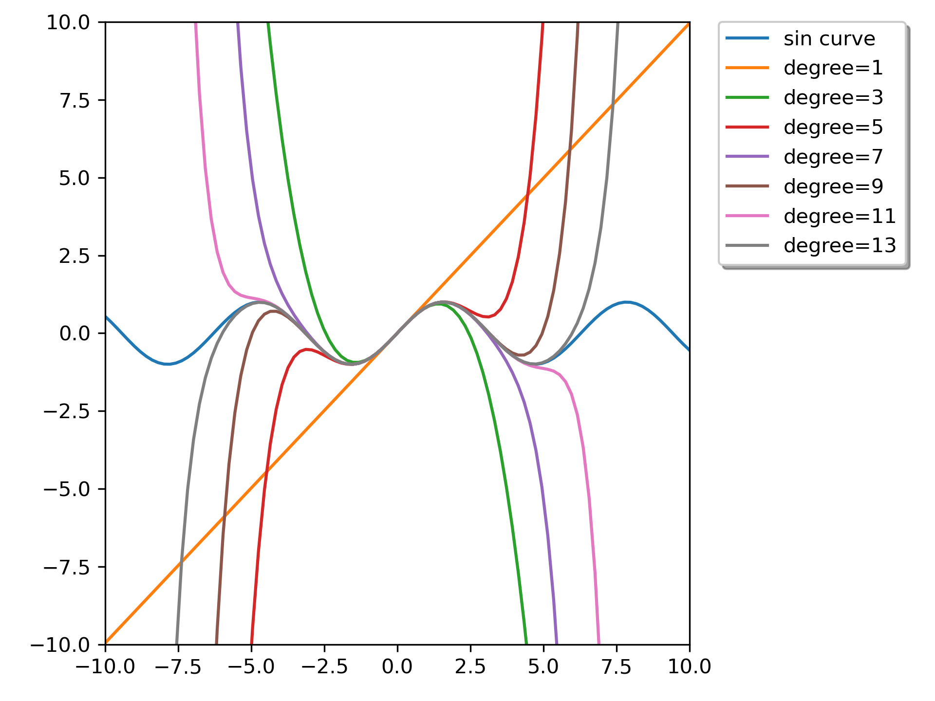
We can calculate Taylor approximation polynomials of sin function with various degrees:
>>> import matplotlib.pyplot as plt
... from scipy.interpolate import approximate_taylor_polynomial
... x = np.linspace(-10.0, 10.0, num=100)
... plt.plot(x, np.sin(x), label="sin curve")
... for degree in np.arange(1, 15, step=2):
...     sin_taylor = approximate_taylor_polynomial(np.sin, 0, degree, 1,
...                                                order=degree + 2)
...     plt.plot(x, sin_taylor(x), label=f"degree={degree}")
... plt.legend(bbox_to_anchor=(1.05, 1), loc='upper left',
...            borderaxespad=0.0, shadow=True)
... plt.tight_layout()
... plt.axis([-10, 10, -10, 10])
... plt.show()
The following pages refer to to this document either explicitly or contain code examples using this.
scipy.interpolate._polyint.approximate_taylor_polynomial
Hover to see nodes names; edges to Self not shown, Caped at 50 nodes.
Using a canvas is more power efficient and can get hundred of nodes ; but does not allow hyperlinks; , arrows or text (beyond on hover)
SVG is more flexible but power hungry; and does not scale well to 50 + nodes.
All aboves nodes referred to, (or are referred from) current nodes; Edges from Self to other have been omitted (or all nodes would be connected to the central node "self" which is not useful). Nodes are colored by the library they belong to, and scaled with the number of references pointing them