splrep(x, y, w=None, xb=None, xe=None, k=3, task=0, s=None, t=None, full_output=0, per=0, quiet=1)
Given the set of data points (x[i], y[i])
determine a smooth spline approximation of degree k on the interval xb <= x <= xe
.
See splev for evaluation of the spline and its derivatives. Uses the FORTRAN routine curfit from FITPACK.
The user is responsible for assuring that the values of x are unique. Otherwise, splrep will not return sensible results.
If provided, knots t must satisfy the Schoenberg-Whitney conditions, i.e., there must be a subset of data points x[j]
such that t[j] < x[j] < t[j+k+1]
, for j=0, 1,...,n-k-2
.
The data points defining a curve y = f(x).
Strictly positive rank-1 array of weights the same length as x and y. The weights are used in computing the weighted least-squares spline fit. If the errors in the y values have standard-deviation given by the vector d, then w should be 1/d. Default is ones(len(x)).
The interval to fit. If None, these default to x[0] and x[-1] respectively.
The order of the spline fit. It is recommended to use cubic splines. Even order splines should be avoided especially with small s values. 1 <= k <= 5
If task==0 find t and c for a given smoothing factor, s.
If task==1 find t and c for another value of the smoothing factor, s. There must have been a previous call with task=0 or task=1 for the same set of data (t will be stored an used internally)
If task=-1 find the weighted least square spline for a given set of knots, t. These should be interior knots as knots on the ends will be added automatically.
A smoothing condition. The amount of smoothness is determined by satisfying the conditions: sum((w * (y - g))**2,axis=0) <= s, where g(x) is the smoothed interpolation of (x,y). The user can use s to control the tradeoff between closeness and smoothness of fit. Larger s means more smoothing while smaller values of s indicate less smoothing. Recommended values of s depend on the weights, w. If the weights represent the inverse of the standard-deviation of y, then a good s value should be found in the range (m-sqrt(2*m),m+sqrt(2*m)) where m is the number of datapoints in x, y, and w. default : s=m-sqrt(2*m) if weights are supplied. s = 0.0 (interpolating) if no weights are supplied.
The knots needed for task=-1. If given then task is automatically set to -1.
If non-zero, then return optional outputs.
If non-zero, data points are considered periodic with period x[m-1] - x[0] and a smooth periodic spline approximation is returned. Values of y[m-1] and w[m-1] are not used.
Non-zero to suppress messages. This parameter is deprecated; use standard Python warning filters instead.
(t,c,k) a tuple containing the vector of knots, the B-spline coefficients, and the degree of the spline.
The weighted sum of squared residuals of the spline approximation.
An integer flag about splrep success. Success is indicated if ier<=0. If ier in [1,2,3] an error occurred but was not raised. Otherwise an error is raised.
A message corresponding to the integer flag, ier.
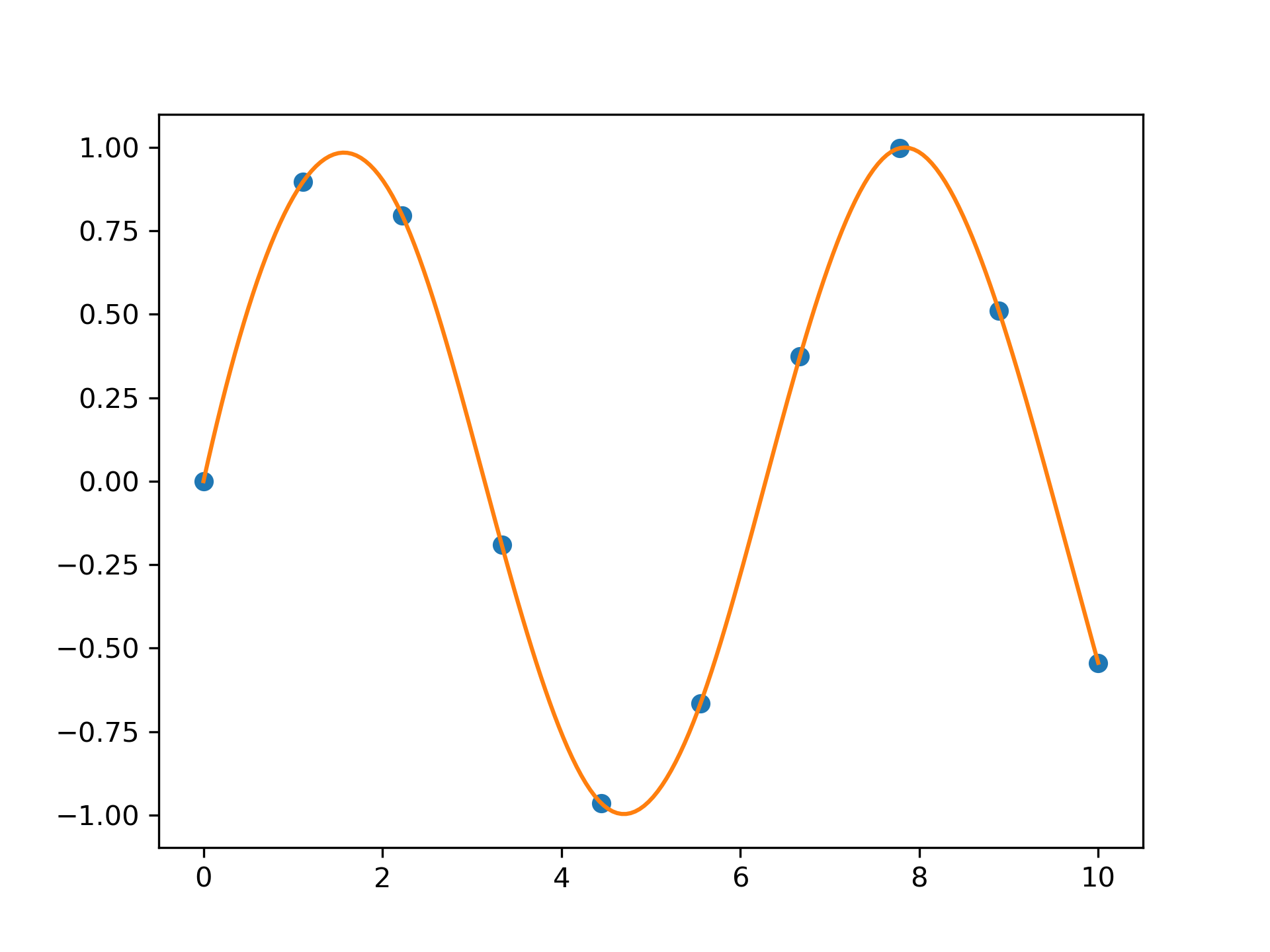
Find the B-spline representation of 1-D curve.
>>> import matplotlib.pyplot as plt
... from scipy.interpolate import splev, splrep
... x = np.linspace(0, 10, 10)
... y = np.sin(x)
... tck = splrep(x, y)
... x2 = np.linspace(0, 10, 200)
... y2 = splev(x2, tck)
... plt.plot(x, y, 'o', x2, y2)
... plt.show()
The following pages refer to to this document either explicitly or contain code examples using this.
scipy.interpolate._fitpack_impl.splint
scipy.interpolate._fitpack_impl.sproot
scipy.interpolate._fitpack_impl.splev
scipy.interpolate._fitpack_impl.splprep
scipy.interpolate._fitpack_impl.bisplrep
Hover to see nodes names; edges to Self not shown, Caped at 50 nodes.
Using a canvas is more power efficient and can get hundred of nodes ; but does not allow hyperlinks; , arrows or text (beyond on hover)
SVG is more flexible but power hungry; and does not scale well to 50 + nodes.
All aboves nodes referred to, (or are referred from) current nodes; Edges from Self to other have been omitted (or all nodes would be connected to the central node "self" which is not useful). Nodes are colored by the library they belong to, and scaled with the number of references pointing them