This function computes the inverse of the 1-D n-point discrete Fourier transform computed by fft
. In other words, ifft(fft(x)) == x
to within numerical accuracy.
The input should be ordered in the same way as is returned by fft
, i.e.,
x[0]
should contain the zero frequency term,
x[1:n//2]
should contain the positive-frequency terms,
x[n//2 + 1:]
should contain the negative-frequency terms, in increasing order starting from the most negative frequency.
For an even number of input points, x[n//2]
represents the sum of the values at the positive and negative Nyquist frequencies, as the two are aliased together. See fft
for details.
If the input parameter n is larger than the size of the input, the input is padded by appending zeros at the end. Even though this is the common approach, it might lead to surprising results. If a different padding is desired, it must be performed before calling ifft
.
If x
is a 1-D array, then the ifft
is equivalent to :
y[k] = np.sum(x * np.exp(2j * np.pi * k * np.arange(n)/n)) / len(x)
As with fft
, ifft
has support for all floating point types and is optimized for real input.
Input array, can be complex.
Length of the transformed axis of the output. If n is smaller than the length of the input, the input is cropped. If it is larger, the input is padded with zeros. If n is not given, the length of the input along the axis specified by :None:None:`axis` is used. See notes about padding issues.
Axis over which to compute the inverse DFT. If not given, the last axis is used.
Normalization mode (see fft
). Default is "backward".
If True, the contents of x can be destroyed; the default is False. See fft
for more details.
Maximum number of workers to use for parallel computation. If negative, the value wraps around from os.cpu_count()
. See ~scipy.fft.fft
for more details.
This argument is reserved for passing in a precomputed plan provided by downstream FFT vendors. It is currently not used in SciPy.
If :None:None:`axes` is larger than the last axis of x.
The truncated or zero-padded input, transformed along the axis indicated by :None:None:`axis`, or the last one if :None:None:`axis` is not specified.
Compute the 1-D inverse discrete Fourier Transform.
fft
The 1-D (forward) FFT, of which :None:None:`ifft` is the inverse.
ifft2
The 2-D inverse FFT.
ifftn
The N-D inverse FFT.
>>> import scipy.fft
... scipy.fft.ifft([0, 4, 0, 0])
array([ 1.+0.j,  0.+1.j, -1.+0.j,  0.-1.j]) # may vary
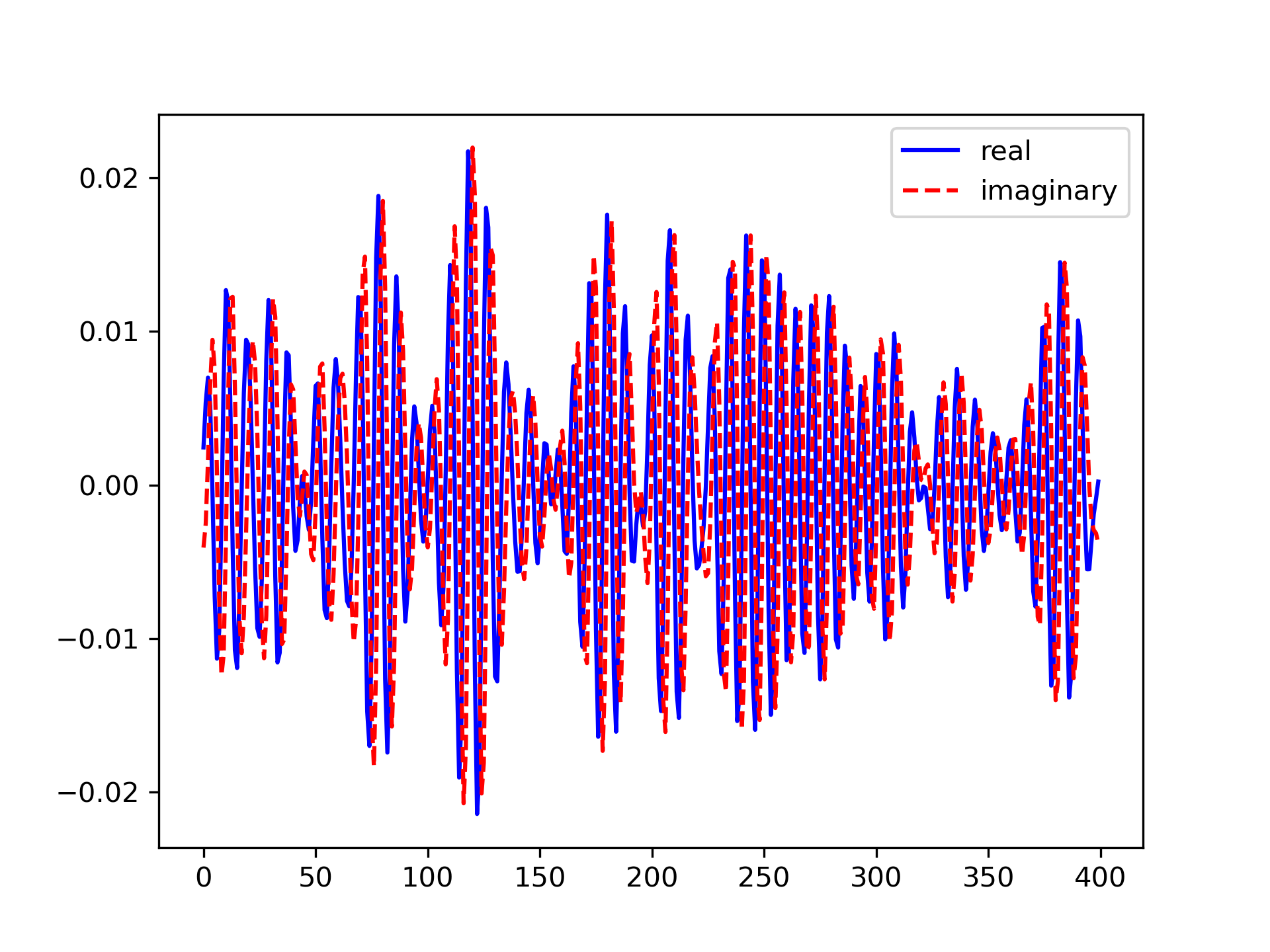
Create and plot a band-limited signal with random phases:
>>> import matplotlib.pyplot as plt
... rng = np.random.default_rng()
... t = np.arange(400)
... n = np.zeros((400,), dtype=complex)
... n[40:60] = np.exp(1j*rng.uniform(0, 2*np.pi, (20,)))
... s = scipy.fft.ifft(n)
... plt.plot(t, s.real, 'b-', t, s.imag, 'r--')
[<matplotlib.lines.Line2D object at ...>, <matplotlib.lines.Line2D object at ...>]
>>> plt.legend(('real', 'imaginary'))
<matplotlib.legend.Legend object at ...>
>>> plt.show()

The following pages refer to to this document either explicitly or contain code examples using this.
scipy.fft._basic.irfft
scipy.fft._helper.next_fast_len
scipy.linalg._basic.solve_circulant
scipy.fft._basic.fft
scipy.fft._basic.ifftn
scipy.fft._basic.ifft
scipy.fft._basic.ifft2
Hover to see nodes names; edges to Self not shown, Caped at 50 nodes.
Using a canvas is more power efficient and can get hundred of nodes ; but does not allow hyperlinks; , arrows or text (beyond on hover)
SVG is more flexible but power hungry; and does not scale well to 50 + nodes.
All aboves nodes referred to, (or are referred from) current nodes; Edges from Self to other have been omitted (or all nodes would be connected to the central node "self" which is not useful). Nodes are colored by the library they belong to, and scaled with the number of references pointing them