peak_prominences(x, peaks, wlen=None)
The prominence of a peak measures how much a peak stands out from the surrounding baseline of the signal and is defined as the vertical distance between the peak and its lowest contour line.
Strategy to compute a peak's prominence:
Extend a horizontal line from the current peak to the left and right until the line either reaches the window border (see wlen
) or intersects the signal again at the slope of a higher peak. An intersection with a peak of the same height is ignored.
On each side find the minimal signal value within the interval defined above. These points are the peak's bases.
The higher one of the two bases marks the peak's lowest contour line. The prominence can then be calculated as the vertical difference between the peaks height itself and its lowest contour line.
Searching for the peak's bases can be slow for large x with periodic behavior because large chunks or even the full signal need to be evaluated for the first algorithmic step. This evaluation area can be limited with the parameter wlen
which restricts the algorithm to a window around the current peak and can shorten the calculation time if the window length is short in relation to x. However, this may stop the algorithm from finding the true global contour line if the peak's true bases are outside this window. Instead, a higher contour line is found within the restricted window leading to a smaller calculated prominence. In practice, this is only relevant for the highest set of peaks in x. This behavior may even be used intentionally to calculate "local" prominences.
A signal with peaks.
Indices of peaks in x.
A window length in samples that optionally limits the evaluated area for each peak to a subset of x. The peak is always placed in the middle of the window therefore the given length is rounded up to the next odd integer. This parameter can speed up the calculation (see Notes).
If a value in :None:None:`peaks` is an invalid index for x.
The calculated prominences for each peak in :None:None:`peaks`.
The peaks' bases as indices in x to the left and right of each peak. The higher base of each pair is a peak's lowest contour line.
Calculate the prominence of each peak in a signal.
For indices in :None:None:`peaks` that don't point to valid local maxima in x, the returned prominence will be 0 and this warning is raised. This also happens if wlen
is smaller than the plateau size of a peak.
find_peaks
Find peaks inside a signal based on peak properties.
peak_widths
Calculate the width of peaks.
>>> from scipy.signal import find_peaks, peak_prominences
... import matplotlib.pyplot as plt
Create a test signal with two overlayed harmonics
>>> x = np.linspace(0, 6 * np.pi, 1000)
... x = np.sin(x) + 0.6 * np.sin(2.6 * x)
Find all peaks and calculate prominences
>>> peaks, _ = find_peaks(x)
... prominences = peak_prominences(x, peaks)[0]
... prominences
array([1.24159486, 0.47840168, 0.28470524, 3.10716793, 0.284603  ,
       0.47822491, 2.48340261, 0.47822491])
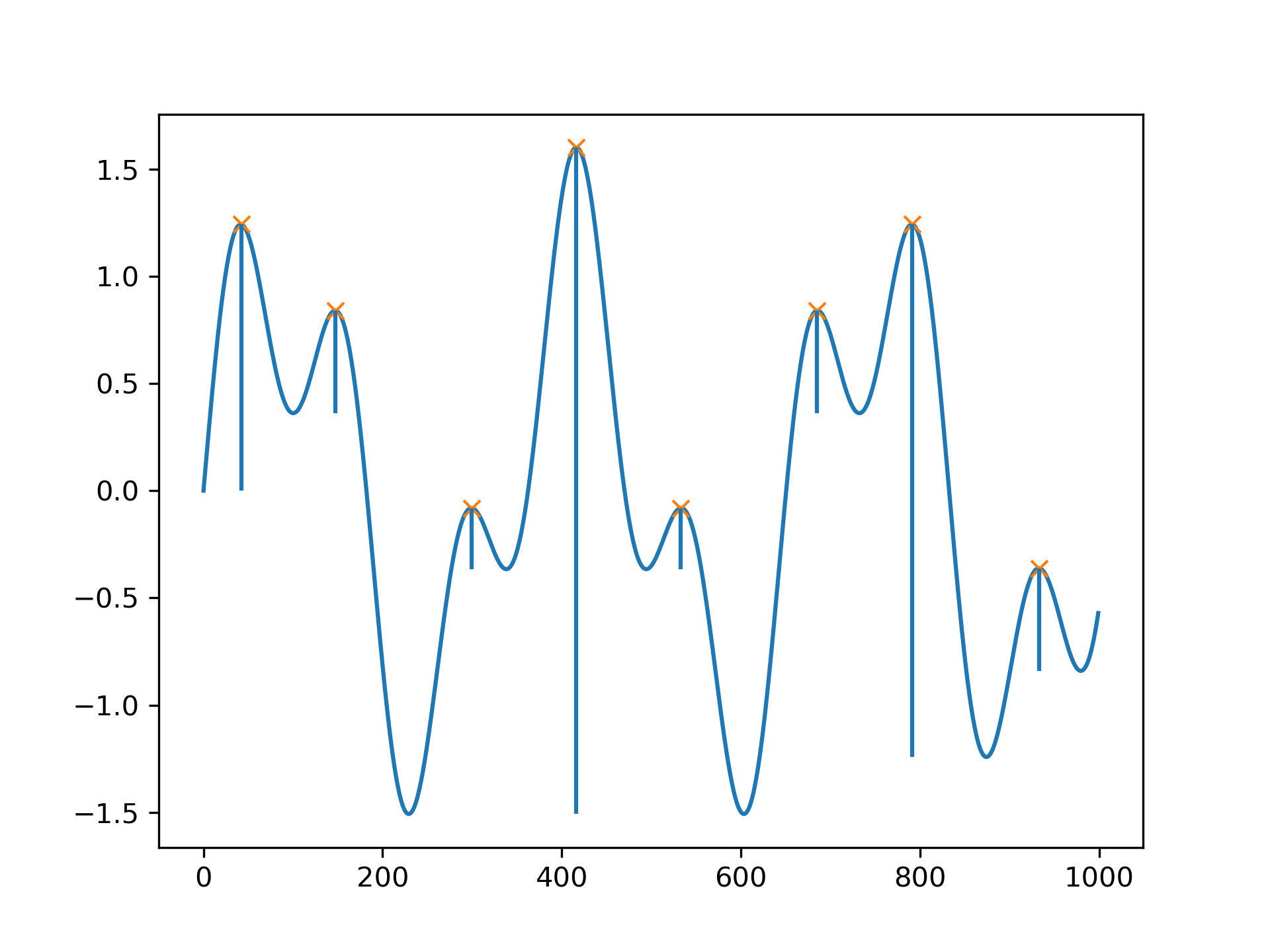
Calculate the height of each peak's contour line and plot the results
>>> contour_heights = x[peaks] - prominences
... plt.plot(x)
... plt.plot(peaks, x[peaks], "x")
... plt.vlines(x=peaks, ymin=contour_heights, ymax=x[peaks])
... plt.show()
Let's evaluate a second example that demonstrates several edge cases for one peak at index 5.
>>> x = np.array([0, 1, 0, 3, 1, 3, 0, 4, 0])
... peaks = np.array([5])
... plt.plot(x)
... plt.plot(peaks, x[peaks], "x")
... plt.show()
... peak_prominences(x, peaks)  # -> (prominences, left_bases, right_bases)
(array([3.]), array([2]), array([6]))
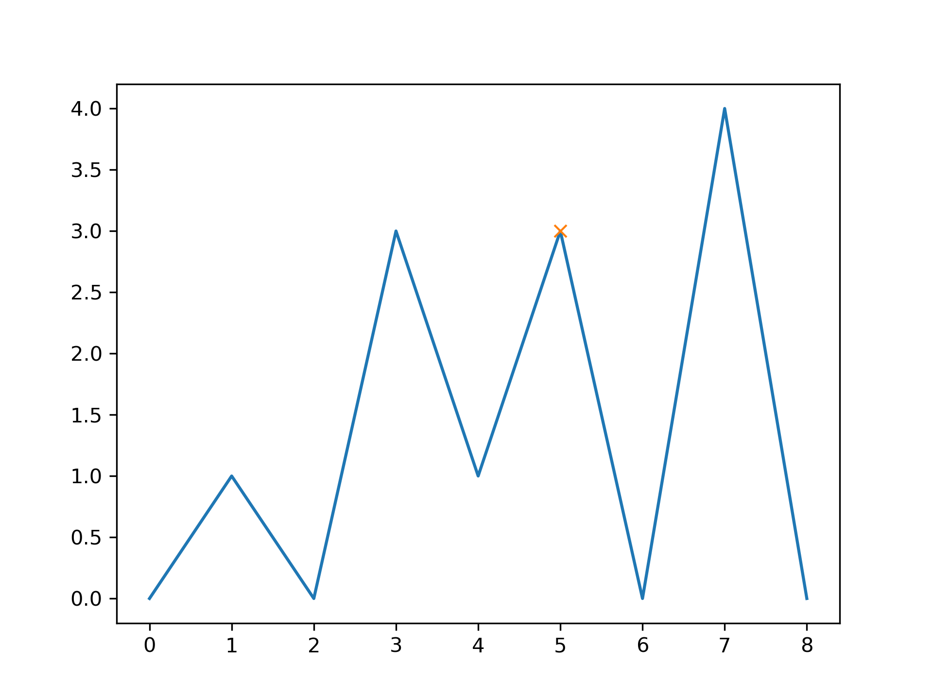
Note how the peak at index 3 of the same height is not considered as a border while searching for the left base. Instead, two minima at 0 and 2 are found in which case the one closer to the evaluated peak is always chosen. On the right side, however, the base must be placed at 6 because the higher peak represents the right border to the evaluated area.
>>> peak_prominences(x, peaks, wlen=3.1)
(array([2.]), array([4]), array([6]))
Here, we restricted the algorithm to a window from 3 to 7 (the length is 5 samples because wlen
was rounded up to the next odd integer). Thus, the only two candidates in the evaluated area are the two neighboring samples and a smaller prominence is calculated.
The following pages refer to to this document either explicitly or contain code examples using this.
scipy.signal._peak_finding_utils._peak_widths
scipy.signal._peak_finding._arg_peaks_as_expected
scipy.signal._peak_finding._arg_x_as_expected
scipy.signal._peak_finding.peak_prominences
scipy.signal._peak_finding._arg_wlen_as_expected
scipy.signal._peak_finding.find_peaks
scipy.signal._peak_finding_utils._peak_prominences
scipy.signal._peak_finding.peak_widths
Hover to see nodes names; edges to Self not shown, Caped at 50 nodes.
Using a canvas is more power efficient and can get hundred of nodes ; but does not allow hyperlinks; , arrows or text (beyond on hover)
SVG is more flexible but power hungry; and does not scale well to 50 + nodes.
All aboves nodes referred to, (or are referred from) current nodes; Edges from Self to other have been omitted (or all nodes would be connected to the central node "self" which is not useful). Nodes are colored by the library they belong to, and scaled with the number of references pointing them