zoom_fft(x, fn, m=None, *, fs=2, endpoint=False, axis=-1)
The defaults are chosen such that signal.zoom_fft(x, 2)
is equivalent to fft.fft(x)
and, if m > len(x)
, that signal.zoom_fft(x, 2, m)
is equivalent to fft.fft(x, m)
.
To graph the magnitude of the resulting transform, use:
plot(linspace(f1, f2, m, endpoint=False), abs(zoom_fft(x, [f1, f2], m)))
If the transform needs to be repeated, use ZoomFFT
to construct a specialized transform function which can be reused without recomputing constants.
The signal to transform.
A length-2 sequence [`f1`, :None:None:`f2`] giving the frequency range, or a scalar, for which the range [0, :None:None:`fn`] is assumed.
The number of points to evaluate. The default is the length of x.
The sampling frequency. If fs=10
represented 10 kHz, for example, then :None:None:`f1` and :None:None:`f2` would also be given in kHz. The default sampling frequency is 2, so :None:None:`f1` and :None:None:`f2` should be in the range [0, 1] to keep the transform below the Nyquist frequency.
If True, :None:None:`f2` is the last sample. Otherwise, it is not included. Default is False.
Axis over which to compute the FFT. If not given, the last axis is used.
The transformed signal. The Fourier transform will be calculated at the points f1, f1+df, f1+2df, ..., f2, where df=(f2-f1)/m.
Compute the DFT of x only for frequencies in range :None:None:`fn`.
ZoomFFT
Class that creates a callable partial FFT function.
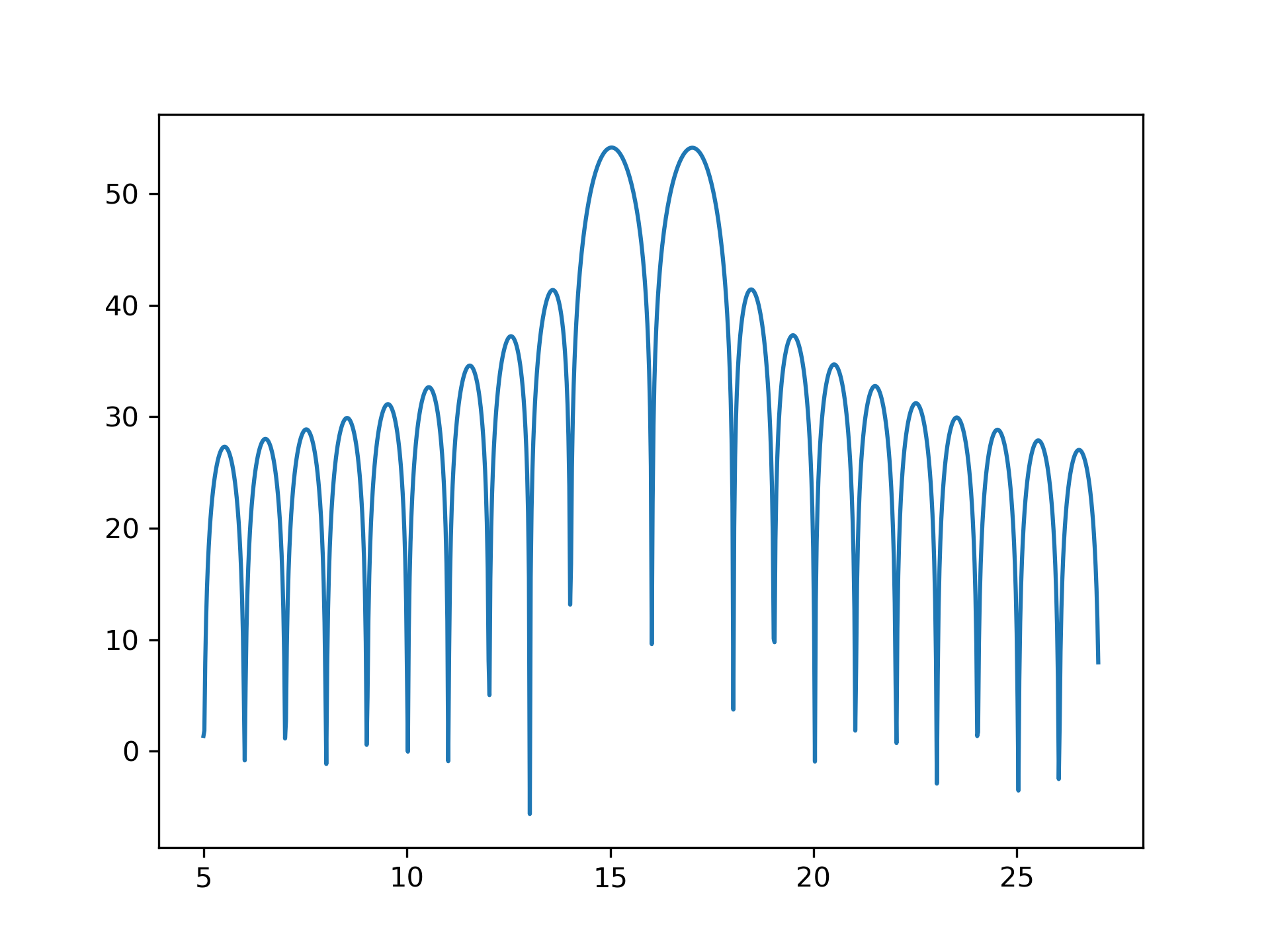
To plot the transform results use something like the following:
>>> from scipy.signal import zoom_fft
... t = np.linspace(0, 1, 1021)
... x = np.cos(2*np.pi*15*t) + np.sin(2*np.pi*17*t)
... f1, f2 = 5, 27
... X = zoom_fft(x, [f1, f2], len(x), fs=1021)
... f = np.linspace(f1, f2, len(x))
... import matplotlib.pyplot as plt
... plt.plot(f, 20*np.log10(np.abs(X)))
... plt.show()
The following pages refer to to this document either explicitly or contain code examples using this.
scipy.signal._czt.CZT
scipy.signal._czt.zoom_fft
scipy.signal._czt.ZoomFFT
Hover to see nodes names; edges to Self not shown, Caped at 50 nodes.
Using a canvas is more power efficient and can get hundred of nodes ; but does not allow hyperlinks; , arrows or text (beyond on hover)
SVG is more flexible but power hungry; and does not scale well to 50 + nodes.
All aboves nodes referred to, (or are referred from) current nodes; Edges from Self to other have been omitted (or all nodes would be connected to the central node "self" which is not useful). Nodes are colored by the library they belong to, and scaled with the number of references pointing them