chebyt(n, monic=False)
Defined to be the solution of
$$(1 - x^2)\frac{d^2}{dx^2}T_n - x\frac{d}{dx}T_n + n^2T_n = 0;$$$T_n$ is a polynomial of degree $n$ .
The polynomials $T_n$ are orthogonal over $[-1, 1]$ with weight function $(1 - x^2)^{-1/2}$ .
Degree of the polynomial.
If :None:None:`True`, scale the leading coefficient to be 1. Default is :None:None:`False`.
Chebyshev polynomial of the first kind.
Chebyshev polynomial of the first kind.
chebyu
Chebyshev polynomial of the second kind.
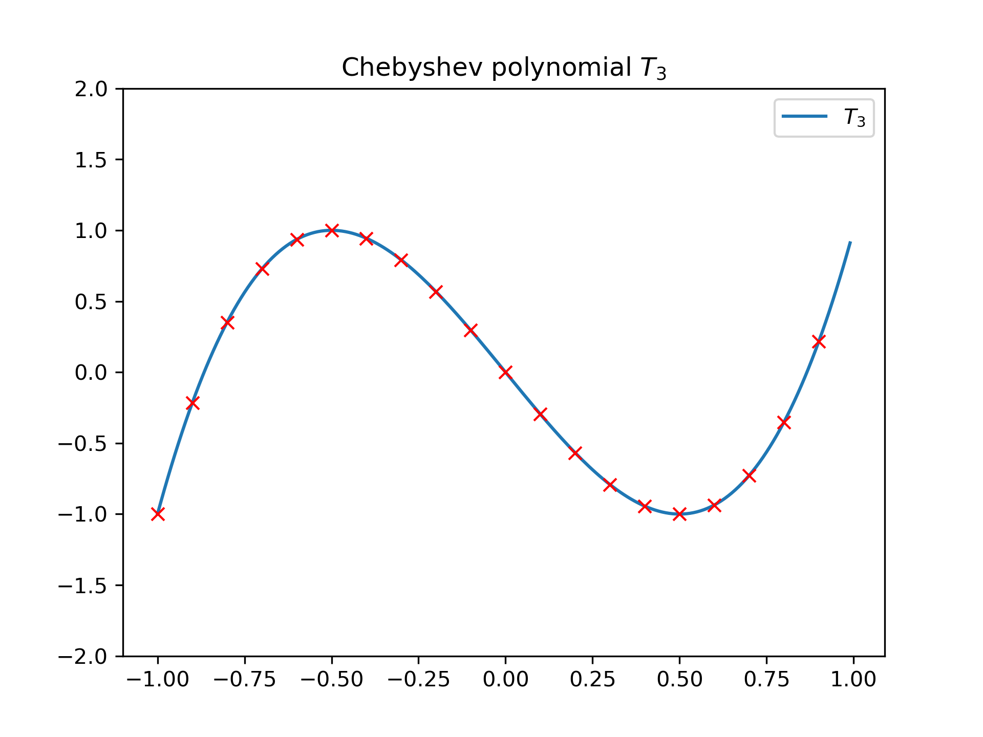
Chebyshev polynomials of the first kind of order $n$ can be obtained as the determinant of specific $n \times n$ matrices. As an example we can check how the points obtained from the determinant of the following $3 \times 3$ matrix lay exacty on $T_3$ :
>>> import matplotlib.pyplot as plt
... from scipy.linalg import det
... from scipy.special import chebyt
... x = np.arange(-1.0, 1.0, 0.01)
... fig, ax = plt.subplots()
... ax.set_ylim(-2.0, 2.0)
... ax.set_title(r'Chebyshev polynomial $T_3$')
... ax.plot(x, chebyt(3)(x), label=rf'$T_3$')
... for p in np.arange(-1.0, 1.0, 0.1):
...     ax.plot(p,
...             det(np.array([[p, 1, 0], [1, 2*p, 1], [0, 1, 2*p]])),
...             'rx')
... plt.legend(loc='best')
... plt.show()
They are also related to the Jacobi Polynomials $P_n^{(-0.5, -0.5)}$ through the relation:
$$P_n^{(-0.5, -0.5)}(x) = \frac{1}{4^n} \binom{2n}{n} T_n(x)$$Let's verify it for $n = 3$ :
>>> from scipy.special import binom
... from scipy.special import chebyt
... from scipy.special import jacobi
... x = np.arange(-1.0, 1.0, 0.01)
... np.allclose(jacobi(3, -0.5, -0.5)(x),
...             1/64 * binom(6, 3) * chebyt(3)(x))
True
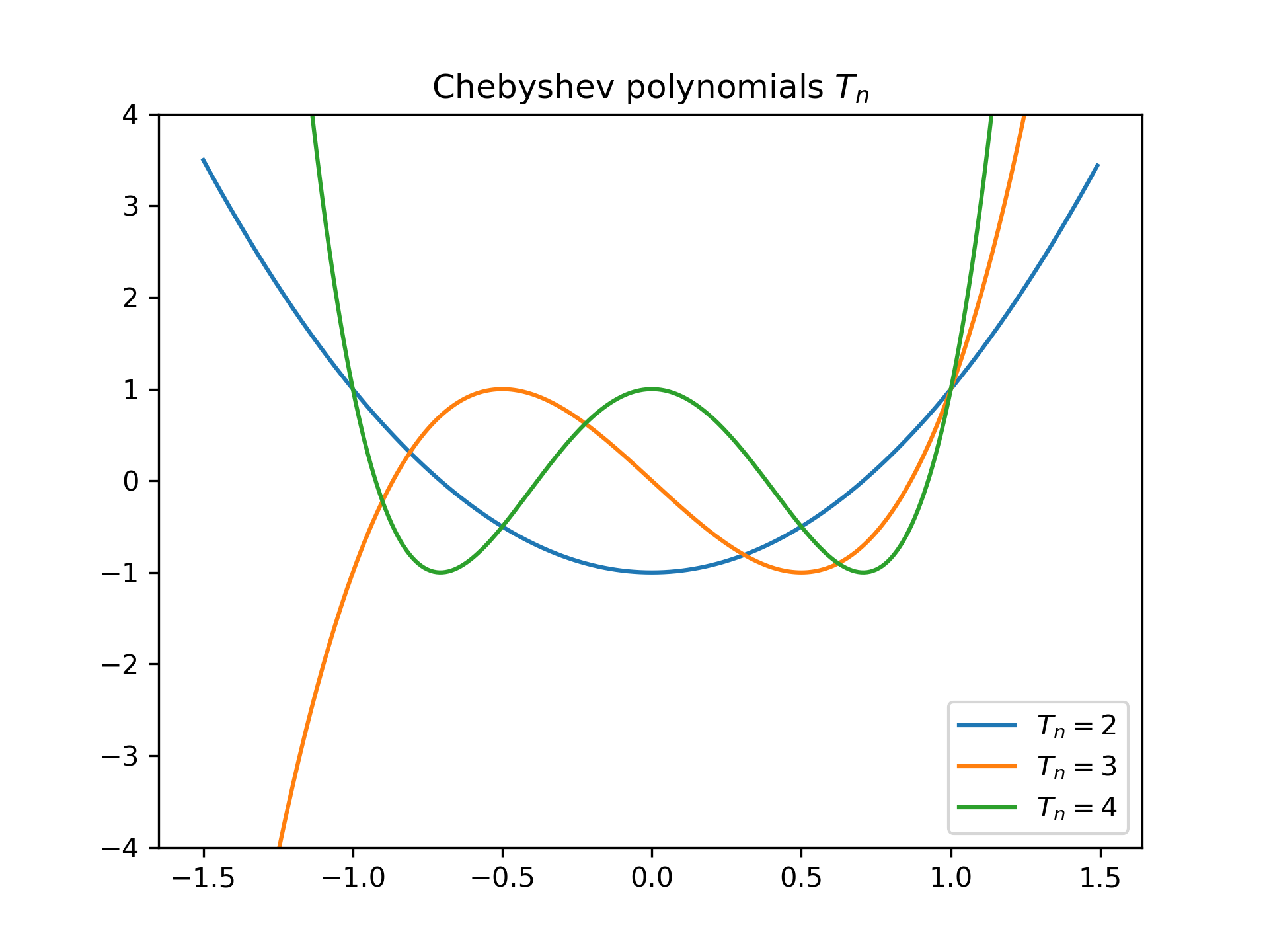
We can plot the Chebyshev polynomials $T_n$ for some values of $n$ :
>>> import matplotlib.pyplot as plt
... from scipy.special import chebyt
... x = np.arange(-1.5, 1.5, 0.01)
... fig, ax = plt.subplots()
... ax.set_ylim(-4.0, 4.0)
... ax.set_title(r'Chebyshev polynomials $T_n$')
... for n in np.arange(2,5):
...     ax.plot(x, chebyt(n)(x), label=rf'$T_n={n}$')
... plt.legend(loc='best')
... plt.show()
The following pages refer to to this document either explicitly or contain code examples using this.
scipy.special._orthogonal.chebyu
scipy.special._orthogonal.chebyc
scipy.special._orthogonal.chebyt
Hover to see nodes names; edges to Self not shown, Caped at 50 nodes.
Using a canvas is more power efficient and can get hundred of nodes ; but does not allow hyperlinks; , arrows or text (beyond on hover)
SVG is more flexible but power hungry; and does not scale well to 50 + nodes.
All aboves nodes referred to, (or are referred from) current nodes; Edges from Self to other have been omitted (or all nodes would be connected to the central node "self" which is not useful). Nodes are colored by the library they belong to, and scaled with the number of references pointing them