max_len_seq(nbits, state=None, length=None, taps=None)
The algorithm for MLS generation is generically described in:
https://en.wikipedia.org/wiki/Maximum_length_sequence
The default values for taps are specifically taken from the first option listed for each value of nbits
in:
https://web.archive.org/web/20181001062252/http://www.newwaveinstruments.com/resources/articles/m_sequence_linear_feedback_shift_register_lfsr.htm
Number of bits to use. Length of the resulting sequence will be (2**nbits) - 1
. Note that generating long sequences (e.g., greater than nbits == 16
) can take a long time.
If array, must be of length nbits
, and will be cast to binary (bool) representation. If None, a seed of ones will be used, producing a repeatable representation. If state
is all zeros, an error is raised as this is invalid. Default: None.
Number of samples to compute. If None, the entire length (2**nbits) - 1
is computed.
Polynomial taps to use (e.g., [7, 6, 1]
for an 8-bit sequence). If None, taps will be automatically selected (for up to nbits == 32
).
Resulting MLS sequence of 0's and 1's.
The final state of the shift register.
Maximum length sequence (MLS) generator.
MLS uses binary convention:
>>> from scipy.signal import max_len_seq
... max_len_seq(4)[0]
array([1, 1, 1, 1, 0, 1, 0, 1, 1, 0, 0, 1, 0, 0, 0], dtype=int8)
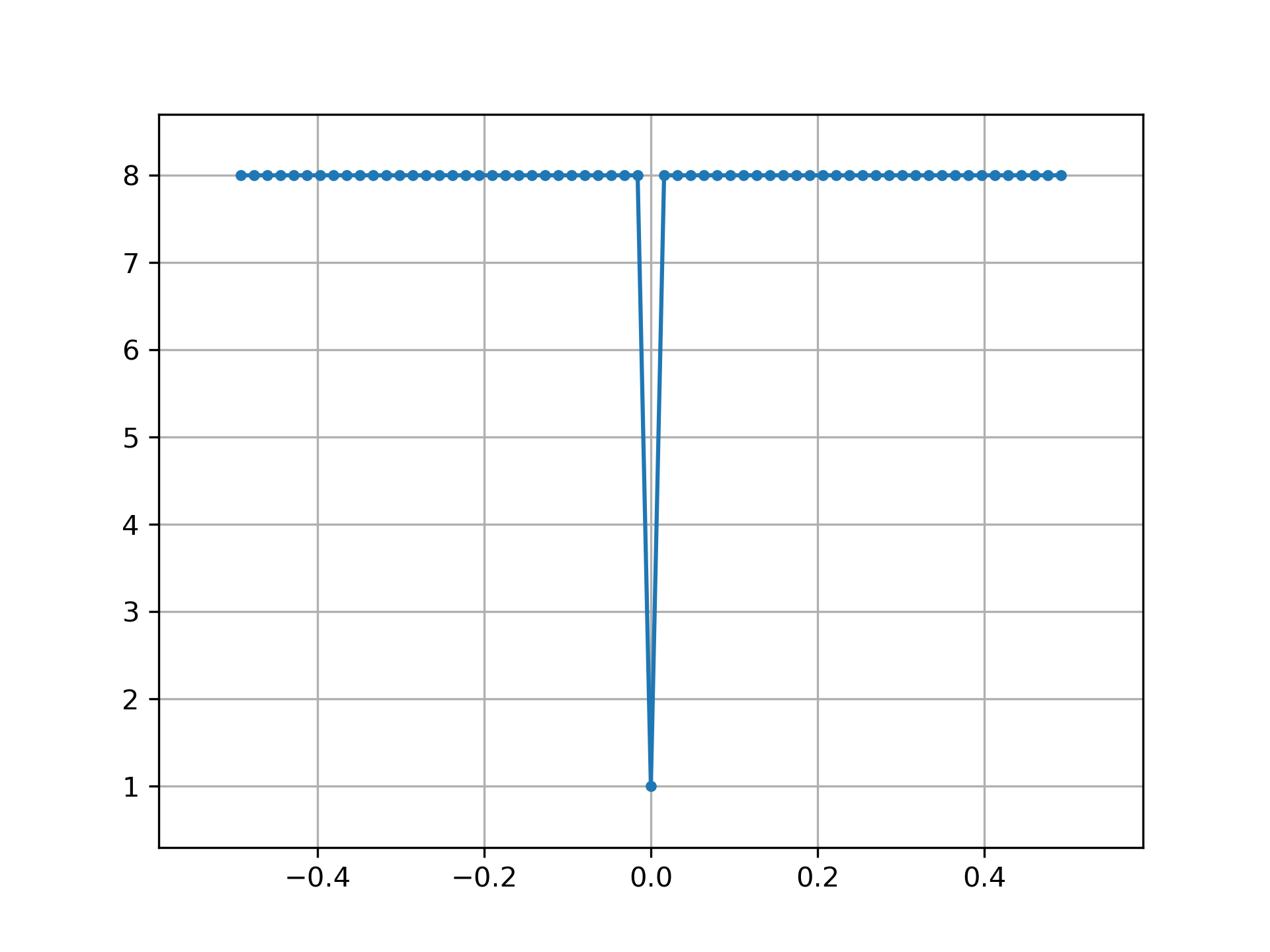
MLS has a white spectrum (except for DC):
>>> import matplotlib.pyplot as plt
... from numpy.fft import fft, ifft, fftshift, fftfreq
... seq = max_len_seq(6)[0]*2-1  # +1 and -1
... spec = fft(seq)
... N = len(seq)
... plt.plot(fftshift(fftfreq(N)), fftshift(np.abs(spec)), '.-')
... plt.margins(0.1, 0.1)
... plt.grid(True)
... plt.show()
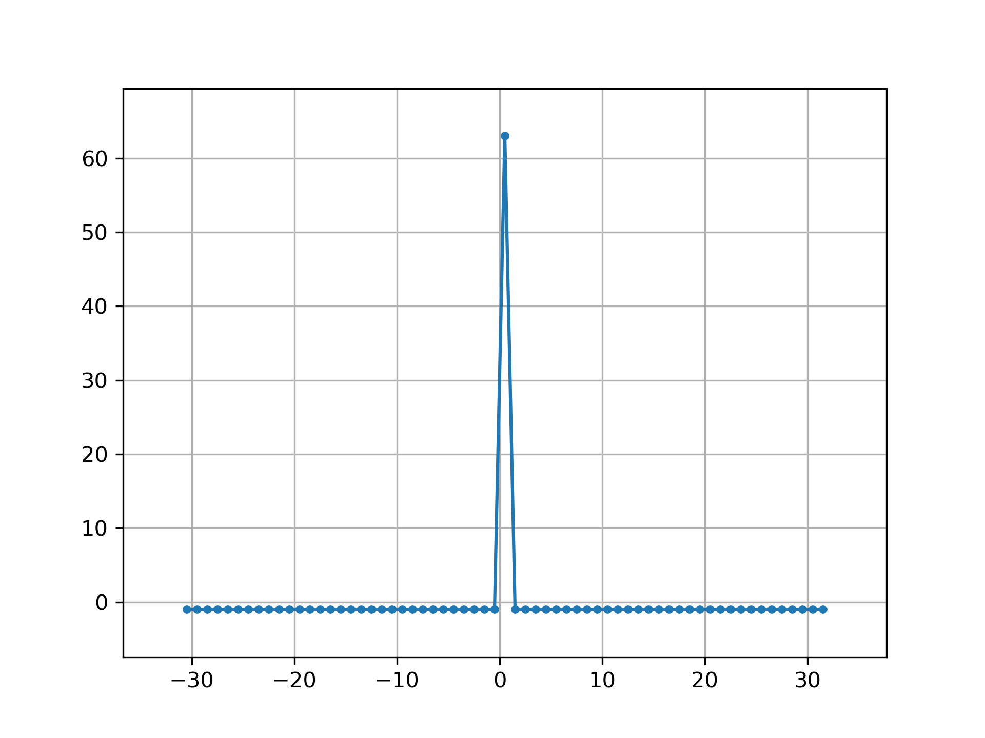
Circular autocorrelation of MLS is an impulse:
>>> acorrcirc = ifft(spec * np.conj(spec)).real
... plt.figure()
... plt.plot(np.arange(-N/2+1, N/2+1), fftshift(acorrcirc), '.-')
... plt.margins(0.1, 0.1)
... plt.grid(True)
... plt.show()
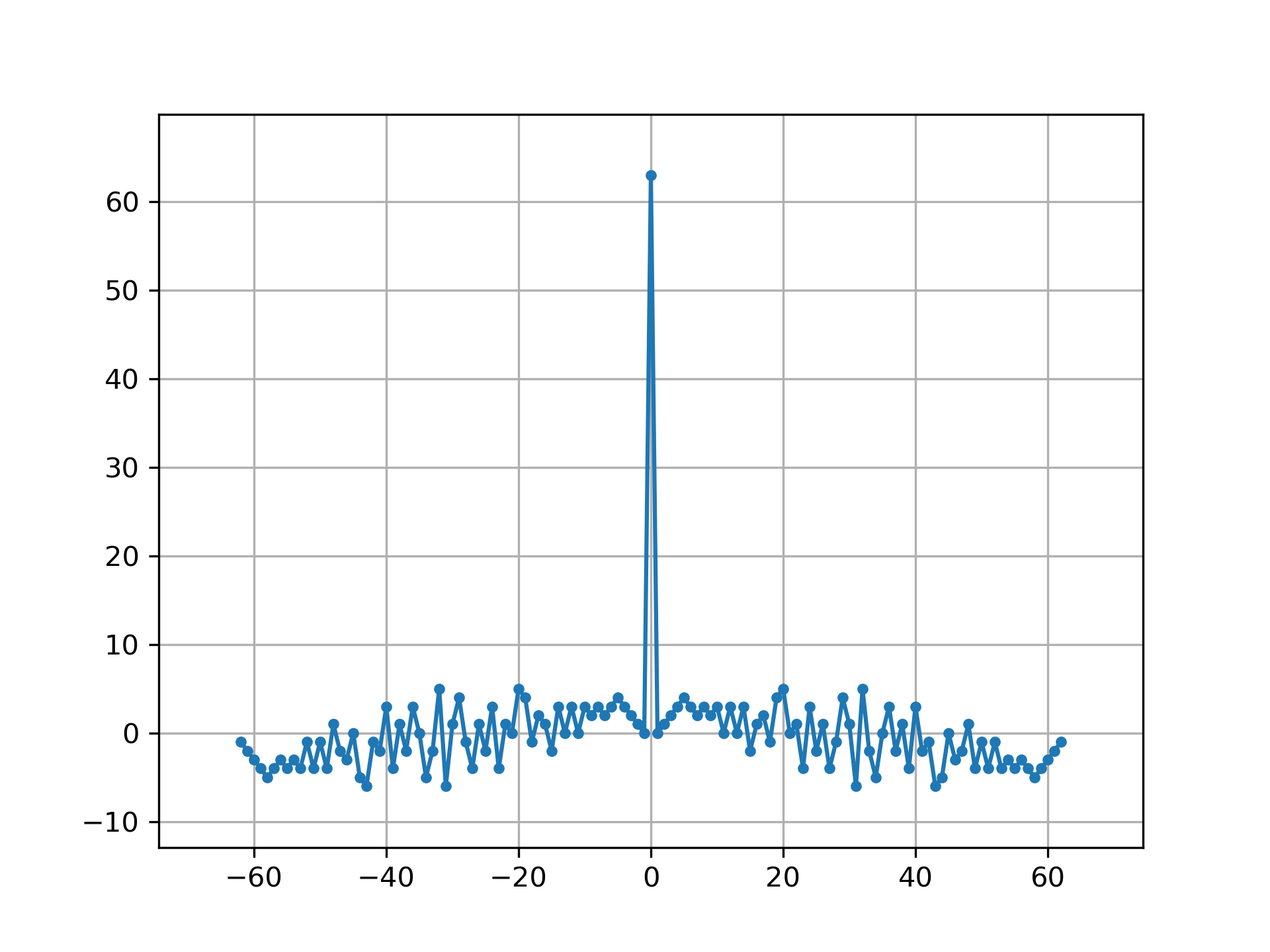
Linear autocorrelation of MLS is approximately an impulse:
>>> acorr = np.correlate(seq, seq, 'full')
... plt.figure()
... plt.plot(np.arange(-N+1, N), acorr, '.-')
... plt.margins(0.1, 0.1)
... plt.grid(True)
... plt.show()
The following pages refer to to this document either explicitly or contain code examples using this.
scipy.signal._max_len_seq.max_len_seq
Hover to see nodes names; edges to Self not shown, Caped at 50 nodes.
Using a canvas is more power efficient and can get hundred of nodes ; but does not allow hyperlinks; , arrows or text (beyond on hover)
SVG is more flexible but power hungry; and does not scale well to 50 + nodes.
All aboves nodes referred to, (or are referred from) current nodes; Edges from Self to other have been omitted (or all nodes would be connected to the central node "self" which is not useful). Nodes are colored by the library they belong to, and scaled with the number of references pointing them