rosen(x)
The function computed is:
sum(100.0*(x[1:] - x[:-1]**2.0)**2.0 + (1 - x[:-1])**2.0)
1-D array of points at which the Rosenbrock function is to be computed.
The value of the Rosenbrock function.
The Rosenbrock function.
>>> from scipy.optimize import rosen
... X = 0.1 * np.arange(10)
... rosen(X)
76.56
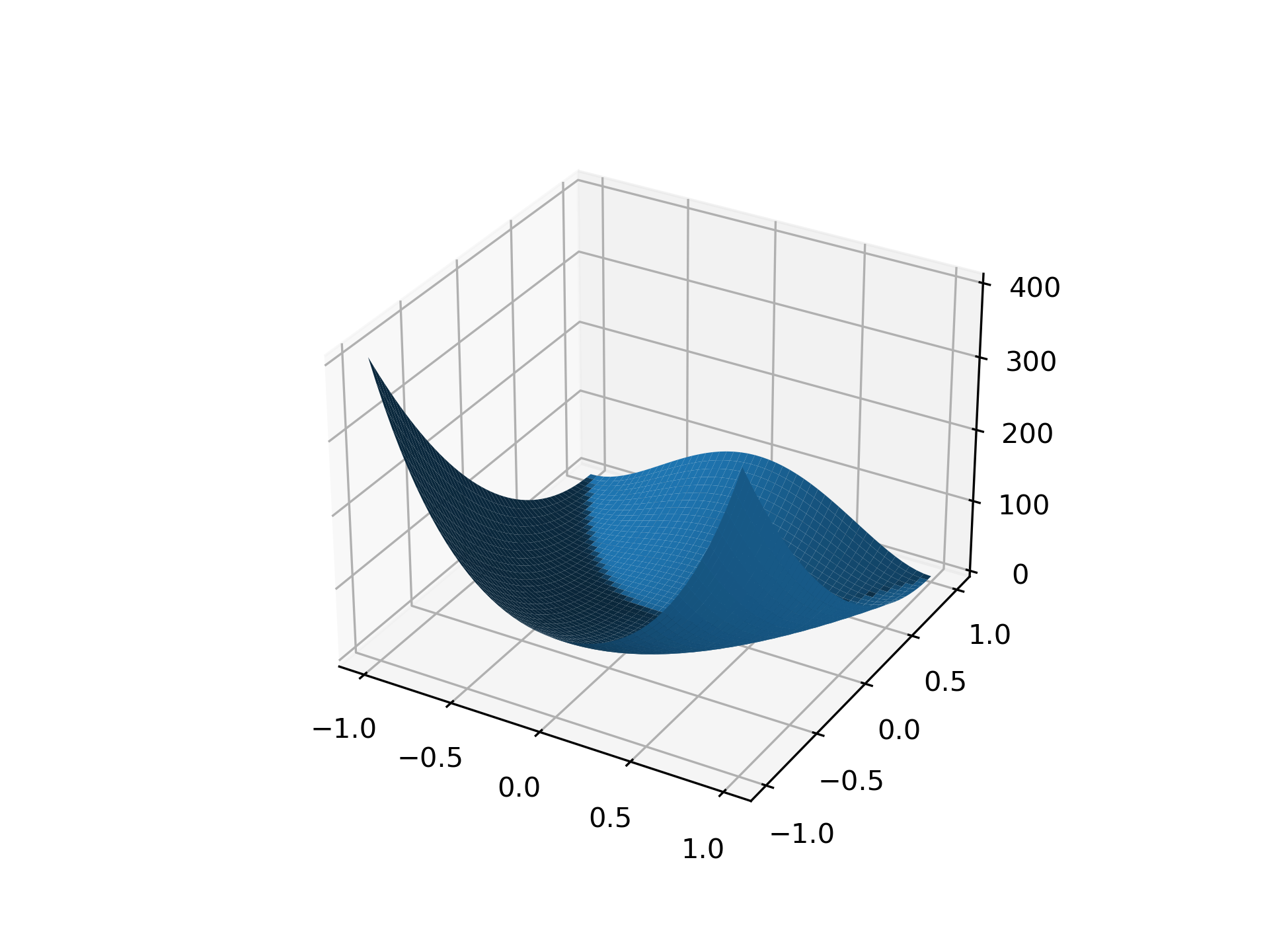
For higher-dimensional input rosen
broadcasts. In the following example, we use this to plot a 2D landscape. Note that rosen_hess
does not broadcast in this manner.
>>> import matplotlib.pyplot as plt
... from mpl_toolkits.mplot3d import Axes3D
... x = np.linspace(-1, 1, 50)
... X, Y = np.meshgrid(x, x)
... ax = plt.subplot(111, projection='3d')
... ax.plot_surface(X, Y, rosen([X, Y]))
... plt.show()
The following pages refer to to this document either explicitly or contain code examples using this.
scipy.optimize._optimize.rosen
scipy.optimize._optimize.rosen_hess
scipy.optimize._optimize.rosen_der
scipy.optimize._minimize.minimize
scipy.optimize._differentialevolution.differential_evolution
scipy.optimize._optimize.rosen_hess_prod
Hover to see nodes names; edges to Self not shown, Caped at 50 nodes.
Using a canvas is more power efficient and can get hundred of nodes ; but does not allow hyperlinks; , arrows or text (beyond on hover)
SVG is more flexible but power hungry; and does not scale well to 50 + nodes.
All aboves nodes referred to, (or are referred from) current nodes; Edges from Self to other have been omitted (or all nodes would be connected to the central node "self" which is not useful). Nodes are colored by the library they belong to, and scaled with the number of references pointing them