An RBF is a scalar valued function in N-dimensional space whose value at $x$ can be expressed in terms of $r=||x - c||$ , where $c$ is the center of the RBF.
An RBF interpolant for the vector of data values $d$ , which are from locations $y$ , is a linear combination of RBFs centered at $y$ plus a polynomial with a specified degree. The RBF interpolant is written as
$$f(x) = K(x, y) a + P(x) b,$$where $K(x, y)$ is a matrix of RBFs with centers at $y$ evaluated at the points $x$ , and $P(x)$ is a matrix of monomials, which span polynomials with the specified degree, evaluated at $x$ . The coefficients $a$ and $b$ are the solution to the linear equations
$$(K(y, y) + \lambda I) a + P(y) b = d$$and
$$P(y)^T a = 0,$$where $\lambda$ is a non-negative smoothing parameter that controls how well we want to fit the data. The data are fit exactly when the smoothing parameter is 0.
The above system is uniquely solvable if the following requirements are met:
$P(y)$ must have full column rank. $P(y)$ always has full column rank when
degreeis -1 or 0. Whendegreeis 1, $P(y)$ has full column rank if the data point locations are not all collinear (N=2), coplanar (N=3), etc.If
kernelis 'multiquadric', 'linear', 'thin_plate_spline', 'cubic', or 'quintic', thendegreemust not be lower than the minimum value listed above.If
smoothingis 0, then each data point location must be distinct.
When using an RBF that is not scale invariant ('multiquadric', 'inverse_multiquadric', 'inverse_quadratic', or 'gaussian'), an appropriate shape parameter must be chosen (e.g., through cross validation). Smaller values for the shape parameter correspond to wider RBFs. The problem can become ill-conditioned or singular when the shape parameter is too small.
The memory required to solve for the RBF interpolation coefficients increases quadratically with the number of data points, which can become impractical when interpolating more than about a thousand data points. To overcome memory limitations for large interpolation problems, the neighbors
argument can be specified to compute an RBF interpolant for each evaluation point using only the nearest data points.
Data point coordinates.
Data values at y.
If specified, the value of the interpolant at each evaluation point will be computed using only this many nearest data points. All the data points are used by default.
Smoothing parameter. The interpolant perfectly fits the data when this is set to 0. For large values, the interpolant approaches a least squares fit of a polynomial with the specified degree. Default is 0.
Type of RBF. This should be one of
Shape parameter that scales the input to the RBF. If kernel
is 'linear', 'thin_plate_spline', 'cubic', or 'quintic', this defaults to 1 and can be ignored because it has the same effect as scaling the smoothing parameter. Otherwise, this must be specified.
Degree of the added polynomial. For some RBFs the interpolant may not be well-posed if the polynomial degree is too small. Those RBFs and their corresponding minimum degrees are
Radial basis function (RBF) interpolation in N dimensions.
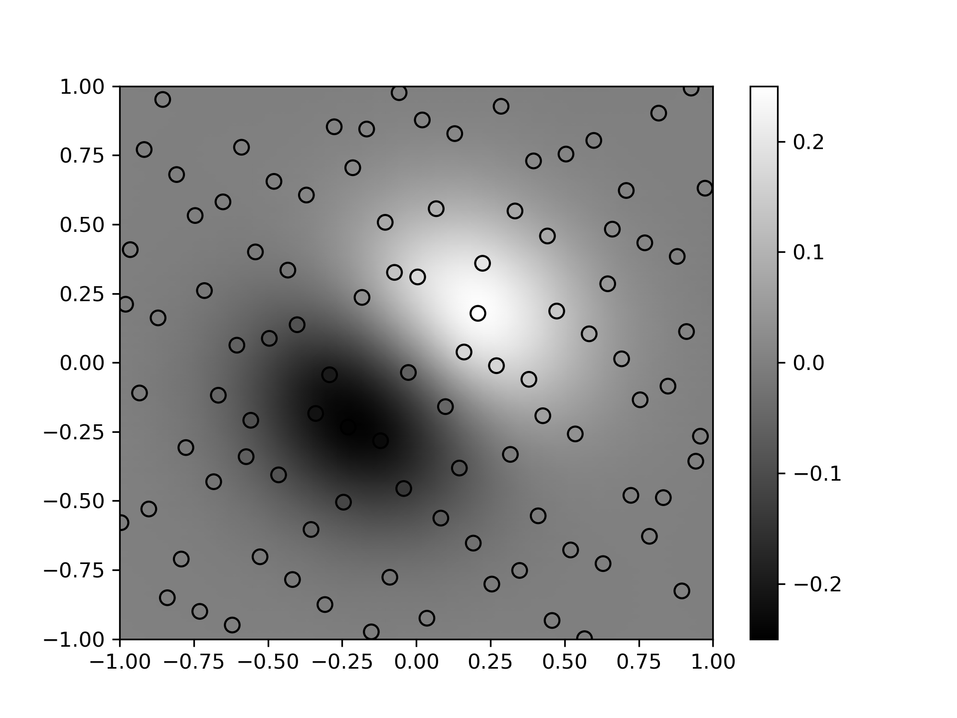
Demonstrate interpolating scattered data to a grid in 2-D.
>>> import matplotlib.pyplot as plt
... from scipy.interpolate import RBFInterpolator
... from scipy.stats.qmc import Halton
>>> rng = np.random.default_rng()
... xobs = 2*Halton(2, seed=rng).random(100) - 1
... yobs = np.sum(xobs, axis=1)*np.exp(-6*np.sum(xobs**2, axis=1))
>>> xgrid = np.mgrid[-1:1:50j, -1:1:50j]
... xflat = xgrid.reshape(2, -1).T
... yflat = RBFInterpolator(xobs, yobs)(xflat)
... ygrid = yflat.reshape(50, 50)
>>> fig, ax = plt.subplots()
... ax.pcolormesh(*xgrid, ygrid, vmin=-0.25, vmax=0.25, shading='gouraud')
... p = ax.scatter(*xobs.T, c=yobs, s=50, ec='k', vmin=-0.25, vmax=0.25)
... fig.colorbar(p)
... plt.show()
The following pages refer to to this document either explicitly or contain code examples using this.
scipy.interpolate._rbf.Rbf
scipy.interpolate._rbfinterp.RBFInterpolator
Hover to see nodes names; edges to Self not shown, Caped at 50 nodes.
Using a canvas is more power efficient and can get hundred of nodes ; but does not allow hyperlinks; , arrows or text (beyond on hover)
SVG is more flexible but power hungry; and does not scale well to 50 + nodes.
All aboves nodes referred to, (or are referred from) current nodes; Edges from Self to other have been omitted (or all nodes would be connected to the central node "self" which is not useful). Nodes are colored by the library they belong to, and scaled with the number of references pointing them