Document

scipy 1.8.0 Pypi GitHub Homepage

newton(func, x0, fprime=None, args=(), tol=1.48e-08, maxiter=50, fprime2=None, x1=None, rtol=0.0, full_output=False, disp=True)

Find a zero of the scalar-valued function :None:None:`func` given a nearby scalar starting point :None:None:`x0`. The Newton-Raphson method is used if the derivative fprime of :None:None:`func` is provided, otherwise the secant method is used. If the second order derivative fprime2 of :None:None:`func` is also provided, then Halley's method is used.

If :None:None:`x0` is a sequence with more than one item, newton returns an array: the zeros of the function from each (scalar) starting point in :None:None:`x0`. In this case, :None:None:`func` must be vectorized to return a sequence or array of the same shape as its first argument. If fprime (fprime2 ) is given, then its return must also have the same shape: each element is the first (second) derivative of :None:None:`func` with respect to its only variable evaluated at each element of its first argument.

newton is for finding roots of a scalar-valued functions of a single variable. For problems involving several variables, see root .

Notes

The convergence rate of the Newton-Raphson method is quadratic, the Halley method is cubic, and the secant method is sub-quadratic. This means that if the function is well-behaved the actual error in the estimated zero after the nth iteration is approximately the square (cube for Halley) of the error after the (n-1)th step. However, the stopping criterion used here is the step size and there is no guarantee that a zero has been found. Consequently, the result should be verified. Safer algorithms are brentq, brenth, ridder, and bisect, but they all require that the root first be bracketed in an interval where the function changes sign. The brentq algorithm is recommended for general use in one dimensional problems when such an interval has been found.

When newton is used with arrays, it is best suited for the following types of problems:

The initial guesses, :None:None:`x0`, are all relatively the same distance from the roots.
Some or all of the extra arguments, :None:None:`args`, are also arrays so that a class of similar problems can be solved together.
The size of the initial guesses, :None:None:`x0`, is larger than O(100) elements. Otherwise, a naive loop may perform as well or better than a vector.

Parameters

func : callable: The function whose zero is wanted. It must be a function of a single variable of the form f(x,a,b,c...) , where a,b,c... are extra arguments that can be passed in the :None:None:`args` parameter.
x0 : float, sequence, or ndarray: An initial estimate of the zero that should be somewhere near the actual zero. If not scalar, then :None:None:`func` must be vectorized and return a sequence or array of the same shape as its first argument.
fprime : callable, optional: The derivative of the function when available and convenient. If it is None (default), then the secant method is used.
args : tuple, optional: Extra arguments to be used in the function call.
tol : float, optional: The allowable error of the zero value. If :None:None:`func` is complex-valued, a larger :None:None:`tol` is recommended as both the real and imaginary parts of x contribute to |x - x0| .
maxiter : int, optional: Maximum number of iterations.
fprime2 : callable, optional: The second order derivative of the function when available and convenient. If it is None (default), then the normal Newton-Raphson or the secant method is used. If it is not None, then Halley's method is used.
x1 : float, optional: Another estimate of the zero that should be somewhere near the actual zero. Used if fprime is not provided.
rtol : float, optional: Tolerance (relative) for termination.
full_output : bool, optional: If :None:None:`full_output` is False (default), the root is returned. If True and :None:None:`x0` is scalar, the return value is (x, r) , where x is the root and r is a RootResults object. If True and :None:None:`x0` is non-scalar, the return value is (x, converged, zero_der) (see Returns section for details).
disp : bool, optional: If True, raise a RuntimeError if the algorithm didn't converge, with the error message containing the number of iterations and current function value. Otherwise, the convergence status is recorded in a RootResults return object. Ignored if :None:None:`x0` is not scalar. Note: this has little to do with displaying, however, the `disp` keyword cannot be renamed for backwards compatibility.

Returns

root : float, sequence, or ndarray: Estimated location where function is zero.
r : `RootResults`, optional: Present if full_output=True and :None:None:`x0` is scalar. Object containing information about the convergence. In particular, r.converged is True if the routine converged.
converged : ndarray of bool, optional: Present if full_output=True and :None:None:`x0` is non-scalar. For vector functions, indicates which elements converged successfully.
zero_der : ndarray of bool, optional: Present if full_output=True and :None:None:`x0` is non-scalar. For vector functions, indicates which elements had a zero derivative.

Find a zero of a real or complex function using the Newton-Raphson (or secant or Halley's) method.

Examples

>>> from scipy import optimize
... import matplotlib.pyplot as plt

>>> def f(x):
...     return (x**3 - 1)  # only one real root at x = 1

fprime is not provided, use the secant method:

>>> root = optimize.newton(f, 1.5)
... root
1.0000000000000016

>>> root = optimize.newton(f, 1.5, fprime2=lambda x: 6 * x)
... root
1.0000000000000016

Only fprime is provided, use the Newton-Raphson method:

>>> root = optimize.newton(f, 1.5, fprime=lambda x: 3 * x**2)
... root
1.0

Both fprime2 and fprime are provided, use Halley's method:

>>> root = optimize.newton(f, 1.5, fprime=lambda x: 3 * x**2,
...                        fprime2=lambda x: 6 * x)
... root
1.0

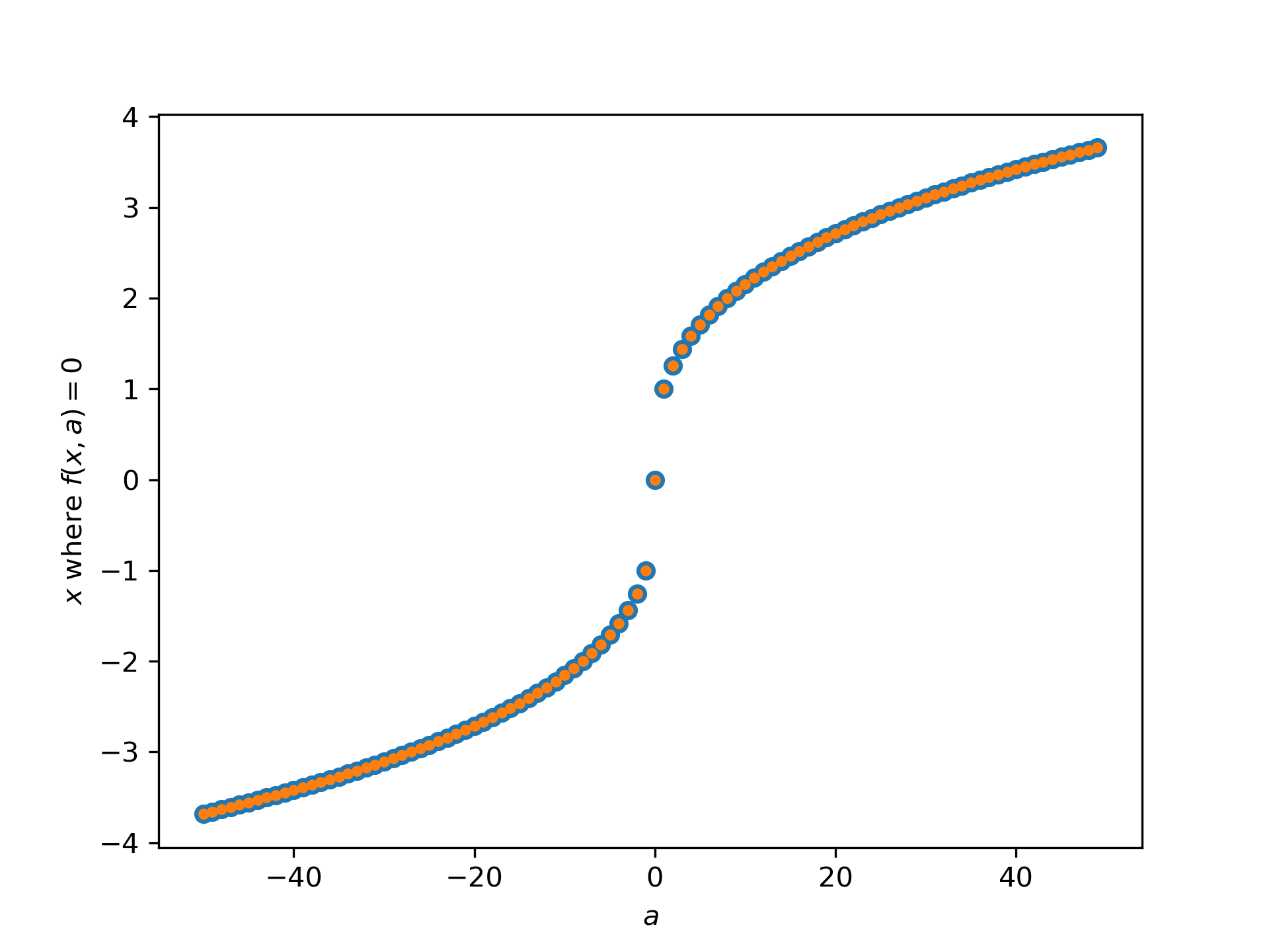
When we want to find zeros for a set of related starting values and/or function parameters, we can provide both of those as an array of inputs:

>>> f = lambda x, a: x**3 - a
... fder = lambda x, a: 3 * x**2
... rng = np.random.default_rng()
... x = rng.standard_normal(100)
... a = np.arange(-50, 50)
... vec_res = optimize.newton(f, x, fprime=fder, args=(a, ), maxiter=200)

The above is the equivalent of solving for each value in (x, a) separately in a for-loop, just faster:

>>> loop_res = [optimize.newton(f, x0, fprime=fder, args=(a0,),
...                             maxiter=200)
...             for x0, a0 in zip(x, a)]
... np.allclose(vec_res, loop_res)
True

Plot the results found for all values of a :

>>> analytical_result = np.sign(a) * np.abs(a)**(1/3)
... fig, ax = plt.subplots()
... ax.plot(a, analytical_result, 'o')
... ax.plot(a, vec_res, '.')
... ax.set_xlabel('$a$')
... ax.set_ylabel('$x$ where $f(x, a)=0$')
... plt.show()

See :

Back References

The following pages refer to to this document either explicitly or contain code examples using this.

scipy.optimize._root_scalar.root_scalar scipy.optimize._zeros_py.bisect scipy.optimize._zeros_py.toms748 scipy.optimize._zeros_py._array_newton scipy.optimize scipy.optimize._zeros_py.newton

Local connectivity graph

Hover to see nodes names; edges to Self not shown, Caped at 50 nodes.

Using a canvas is more power efficient and can get hundred of nodes ; but does not allow hyperlinks; , arrows or text (beyond on hover)

SVG is more flexible but power hungry; and does not scale well to 50 + nodes.

All aboves nodes referred to, (or are referred from) current nodes; Edges from Self to other have been omitted (or all nodes would be connected to the central node "self" which is not useful). Nodes are colored by the library they belong to, and scaled with the number of references pointing them