This function computes the 1-D n-point discrete Fourier Transform (DFT) with the efficient Fast Fourier Transform (FFT) algorithm .
FFT (Fast Fourier Transform) refers to a way the discrete Fourier Transform (DFT) can be calculated efficiently, by using symmetries in the calculated terms. The symmetry is highest when n is a power of 2, and the transform is therefore most efficient for these sizes. For poorly factorizable sizes, scipy.fft
uses Bluestein's algorithm and so is never worse than O(n log n). Further performance improvements may be seen by zero-padding the input using next_fast_len
.
If x
is a 1d array, then the fft
is equivalent to :
y[k] = np.sum(x * np.exp(-2j * np.pi * k * np.arange(n)/n))
The frequency term f=k/n
is found at y[k]
. At y[n/2]
we reach the Nyquist frequency and wrap around to the negative-frequency terms. So, for an 8-point transform, the frequencies of the result are [0, 1, 2, 3, -4, -3, -2, -1]. To rearrange the fft output so that the zero-frequency component is centered, like [-4, -3, -2, -1, 0, 1, 2, 3], use :None:None:`fftshift`.
Transforms can be done in single, double, or extended precision (long double) floating point. Half precision inputs will be converted to single precision and non-floating-point inputs will be converted to double precision.
If the data type of x
is real, a "real FFT" algorithm is automatically used, which roughly halves the computation time. To increase efficiency a little further, use rfft
, which does the same calculation, but only outputs half of the symmetrical spectrum. If the data are both real and symmetrical, the :None:None:`dct` can again double the efficiency, by generating half of the spectrum from half of the signal.
When overwrite_x=True
is specified, the memory referenced by x
may be used by the implementation in any way. This may include reusing the memory for the result, but this is in no way guaranteed. You should not rely on the contents of x
after the transform as this may change in future without warning.
The workers
argument specifies the maximum number of parallel jobs to split the FFT computation into. This will execute independent 1-D FFTs within x
. So, x
must be at least 2-D and the non-transformed axes must be large enough to split into chunks. If x
is too small, fewer jobs may be used than requested.
Input array, can be complex.
Length of the transformed axis of the output. If n is smaller than the length of the input, the input is cropped. If it is larger, the input is padded with zeros. If n is not given, the length of the input along the axis specified by :None:None:`axis` is used.
Axis over which to compute the FFT. If not given, the last axis is used.
Normalization mode. Default is "backward", meaning no normalization on the forward transforms and scaling by 1/n
on the ifft
. "forward" instead applies the 1/n
factor on the forward tranform. For norm="ortho"
, both directions are scaled by 1/sqrt(n)
.
norm={"forward", "backward"}
options were added
If True, the contents of x can be destroyed; the default is False. See the notes below for more details.
Maximum number of workers to use for parallel computation. If negative, the value wraps around from os.cpu_count()
. See below for more details.
This argument is reserved for passing in a precomputed plan provided by downstream FFT vendors. It is currently not used in SciPy.
if :None:None:`axes` is larger than the last axis of x.
The truncated or zero-padded input, transformed along the axis indicated by :None:None:`axis`, or the last one if :None:None:`axis` is not specified.
Compute the 1-D discrete Fourier Transform.
fft2
The 2-D FFT.
fftfreq
Frequency bins for given FFT parameters.
fftn
The N-D FFT.
ifft
The inverse of :None:None:`fft`.
next_fast_len
Size to pad input to for most efficient transforms
rfftn
The N-D FFT of real input.
>>> import scipy.fft
... scipy.fft.fft(np.exp(2j * np.pi * np.arange(8) / 8))
array([-2.33486982e-16+1.14423775e-17j,  8.00000000e+00-1.25557246e-15j,
        2.33486982e-16+2.33486982e-16j,  0.00000000e+00+1.22464680e-16j,
       -1.14423775e-17+2.33486982e-16j,  0.00000000e+00+5.20784380e-16j,
        1.14423775e-17+1.14423775e-17j,  0.00000000e+00+1.22464680e-16j])
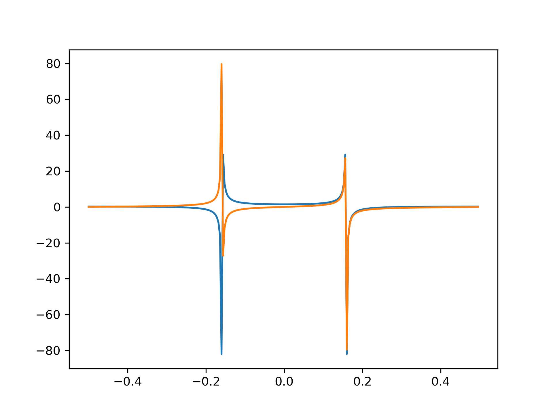
In this example, real input has an FFT which is Hermitian, i.e., symmetric in the real part and anti-symmetric in the imaginary part:
>>> from scipy.fft import fft, fftfreq, fftshift
... import matplotlib.pyplot as plt
... t = np.arange(256)
... sp = fftshift(fft(np.sin(t)))
... freq = fftshift(fftfreq(t.shape[-1]))
... plt.plot(freq, sp.real, freq, sp.imag)
[<matplotlib.lines.Line2D object at 0x...>, <matplotlib.lines.Line2D object at 0x...>]
>>> plt.show()
The following pages refer to to this document either explicitly or contain code examples using this.
scipy.signal._signaltools.resample
scipy.linalg._special_matrices.dft
scipy.signal.windows._windows.general_hamming
Hover to see nodes names; edges to Self not shown, Caped at 50 nodes.
Using a canvas is more power efficient and can get hundred of nodes ; but does not allow hyperlinks; , arrows or text (beyond on hover)
SVG is more flexible but power hungry; and does not scale well to 50 + nodes.
All aboves nodes referred to, (or are referred from) current nodes; Edges from Self to other have been omitted (or all nodes would be connected to the central node "self" which is not useful). Nodes are colored by the library they belong to, and scaled with the number of references pointing them