geometric_slerp(start: 'npt.ArrayLike', end: 'npt.ArrayLike', t: 'npt.ArrayLike', tol: 'float' = 1e-07) -> 'np.ndarray'
The interpolation occurs along a unit-radius great circle arc in arbitrary dimensional space.
The implementation is based on the mathematical formula provided in , and the first known presentation of this algorithm, derived from study of 4-D geometry, is credited to Glenn Davis in a footnote of the original quaternion Slerp publication by Ken Shoemake .
Single n-dimensional input coordinate in a 1-D array-like object. n must be greater than 1.
Single n-dimensional input coordinate in a 1-D array-like object. n must be greater than 1.
A float or 1D array-like of doubles representing interpolation parameters, with values required in the inclusive interval between 0 and 1. A common approach is to generate the array with np.linspace(0, 1, n_pts)
for linearly spaced points. Ascending, descending, and scrambled orders are permitted.
The absolute tolerance for determining if the start and end coordinates are antipodes.
If start
and end
are antipodes, not on the unit n-sphere, or for a variety of degenerate conditions.
An array of doubles containing the interpolated spherical path and including start and end when 0 and 1 t are used. The interpolated values should correspond to the same sort order provided in the t array. The result may be 1-dimensional if t
is a float.
Geometric spherical linear interpolation.
scipy.spatial.transform.Slerp
3-D Slerp that works with quaternions
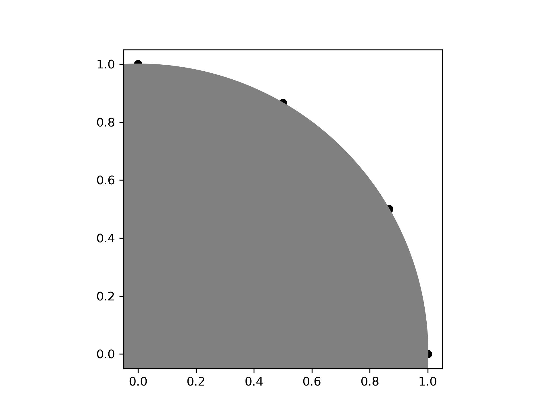
Interpolate four linearly-spaced values on the circumference of a circle spanning 90 degrees:
>>> from scipy.spatial import geometric_slerp
... import matplotlib.pyplot as plt
... fig = plt.figure()
... ax = fig.add_subplot(111)
... start = np.array([1, 0])
... end = np.array([0, 1])
... t_vals = np.linspace(0, 1, 4)
... result = geometric_slerp(start,
...                          end,
...                          t_vals)
The interpolated results should be at 30 degree intervals recognizable on the unit circle:
>>> ax.scatter(result[...,0], result[...,1], c='k')
... circle = plt.Circle((0, 0), 1, color='grey')
... ax.add_artist(circle)
... ax.set_aspect('equal')
... plt.show()
Attempting to interpolate between antipodes on a circle is ambiguous because there are two possible paths, and on a sphere there are infinite possible paths on the geodesic surface. Nonetheless, one of the ambiguous paths is returned along with a warning:
>>> opposite_pole = np.array([-1, 0])
... with np.testing.suppress_warnings() as sup:
...     sup.filter(UserWarning)
...     geometric_slerp(start,
...                     opposite_pole,
...                     t_vals)
array([[ 1.00000000e+00,  0.00000000e+00],
       [ 5.00000000e-01,  8.66025404e-01],
       [-5.00000000e-01,  8.66025404e-01],
       [-1.00000000e+00,  1.22464680e-16]])
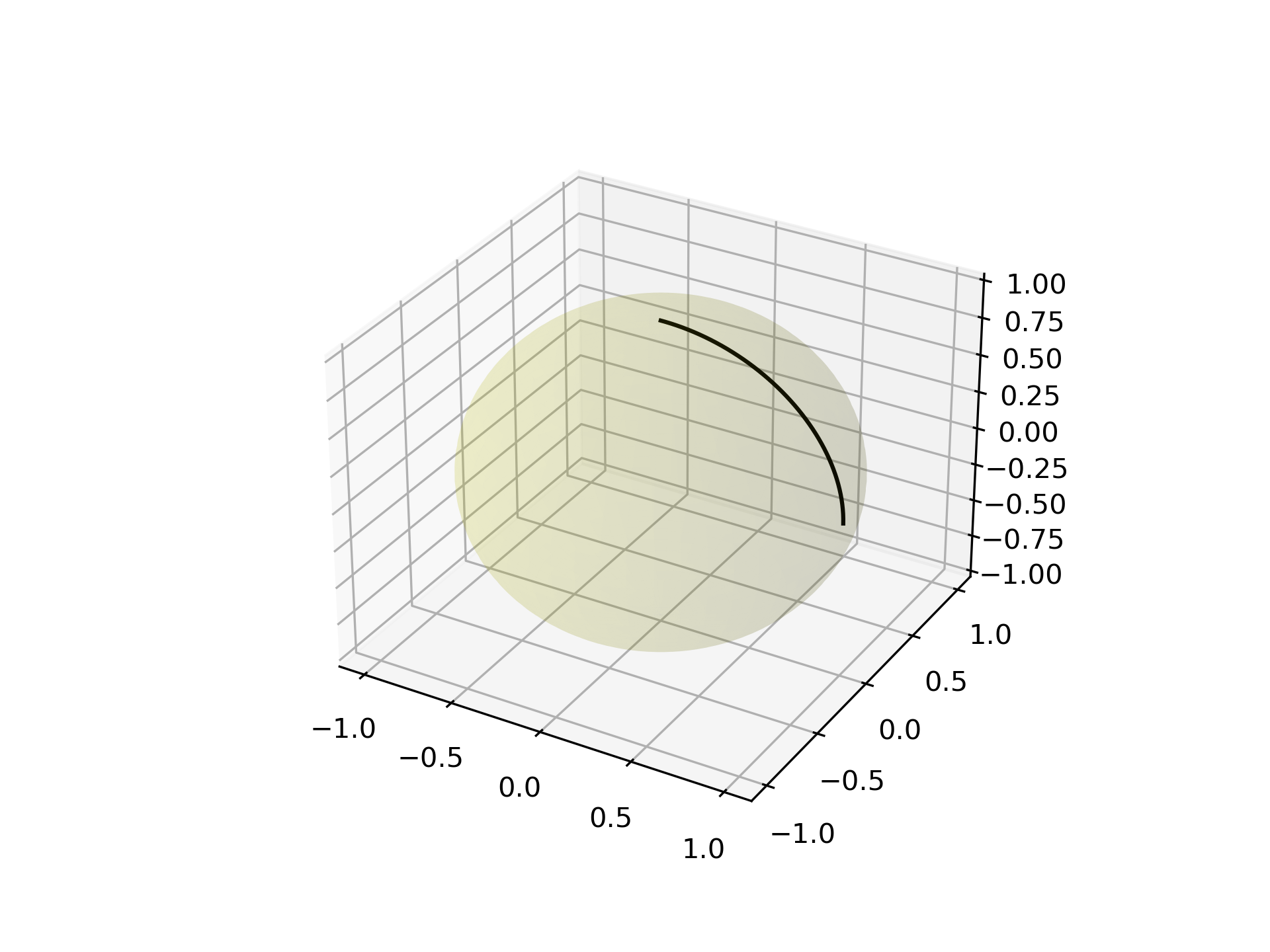
Extend the original example to a sphere and plot interpolation points in 3D:
>>> from mpl_toolkits.mplot3d import proj3d
... fig = plt.figure()
... ax = fig.add_subplot(111, projection='3d')
Plot the unit sphere for reference (optional):
>>> u = np.linspace(0, 2 * np.pi, 100)
... v = np.linspace(0, np.pi, 100)
... x = np.outer(np.cos(u), np.sin(v))
... y = np.outer(np.sin(u), np.sin(v))
... z = np.outer(np.ones(np.size(u)), np.cos(v))
... ax.plot_surface(x, y, z, color='y', alpha=0.1)
Interpolating over a larger number of points may provide the appearance of a smooth curve on the surface of the sphere, which is also useful for discretized integration calculations on a sphere surface:
>>> start = np.array([1, 0, 0])
... end = np.array([0, 0, 1])
... t_vals = np.linspace(0, 1, 200)
... result = geometric_slerp(start,
...                          end,
...                          t_vals)
... ax.plot(result[...,0],
...         result[...,1],
...         result[...,2],
...         c='k')
... plt.show()
The following pages refer to to this document either explicitly or contain code examples using this.
scipy.spatial._geometric_slerp.geometric_slerp
Hover to see nodes names; edges to Self not shown, Caped at 50 nodes.
Using a canvas is more power efficient and can get hundred of nodes ; but does not allow hyperlinks; , arrows or text (beyond on hover)
SVG is more flexible but power hungry; and does not scale well to 50 + nodes.
All aboves nodes referred to, (or are referred from) current nodes; Edges from Self to other have been omitted (or all nodes would be connected to the central node "self" which is not useful). Nodes are colored by the library they belong to, and scaled with the number of references pointing them