griddata(points, values, xi, method='linear', fill_value=nan, rescale=False)
Data point coordinates.
Data values.
Points at which to interpolate data.
Method of interpolation. One of
nearest
return the value at the data point closest to the point of interpolation. See NearestNDInterpolator
for more details.
linear
tessellate the input point set to N-D simplices, and interpolate linearly on each simplex. See LinearNDInterpolator
for more details.
cubic
(1-D)
return the value determined from a cubic spline.
cubic
(2-D)
return the value determined from a piecewise cubic, continuously differentiable (C1), and approximately curvature-minimizing polynomial surface. See CloughTocher2DInterpolator
for more details.
Value used to fill in for requested points outside of the convex hull of the input points. If not provided, then the default is nan
. This option has no effect for the 'nearest' method.
Rescale points to unit cube before performing interpolation. This is useful if some of the input dimensions have incommensurable units and differ by many orders of magnitude.
Array of interpolated values.
Interpolate unstructured D-D data.
CloughTocher2DInterpolator
Piecewise cubic, C1 smooth, curvature-minimizing interpolant in 2D.
LinearNDInterpolator
Piecewise linear interpolant in N dimensions.
NearestNDInterpolator
Nearest-neighbor interpolation in N dimensions.
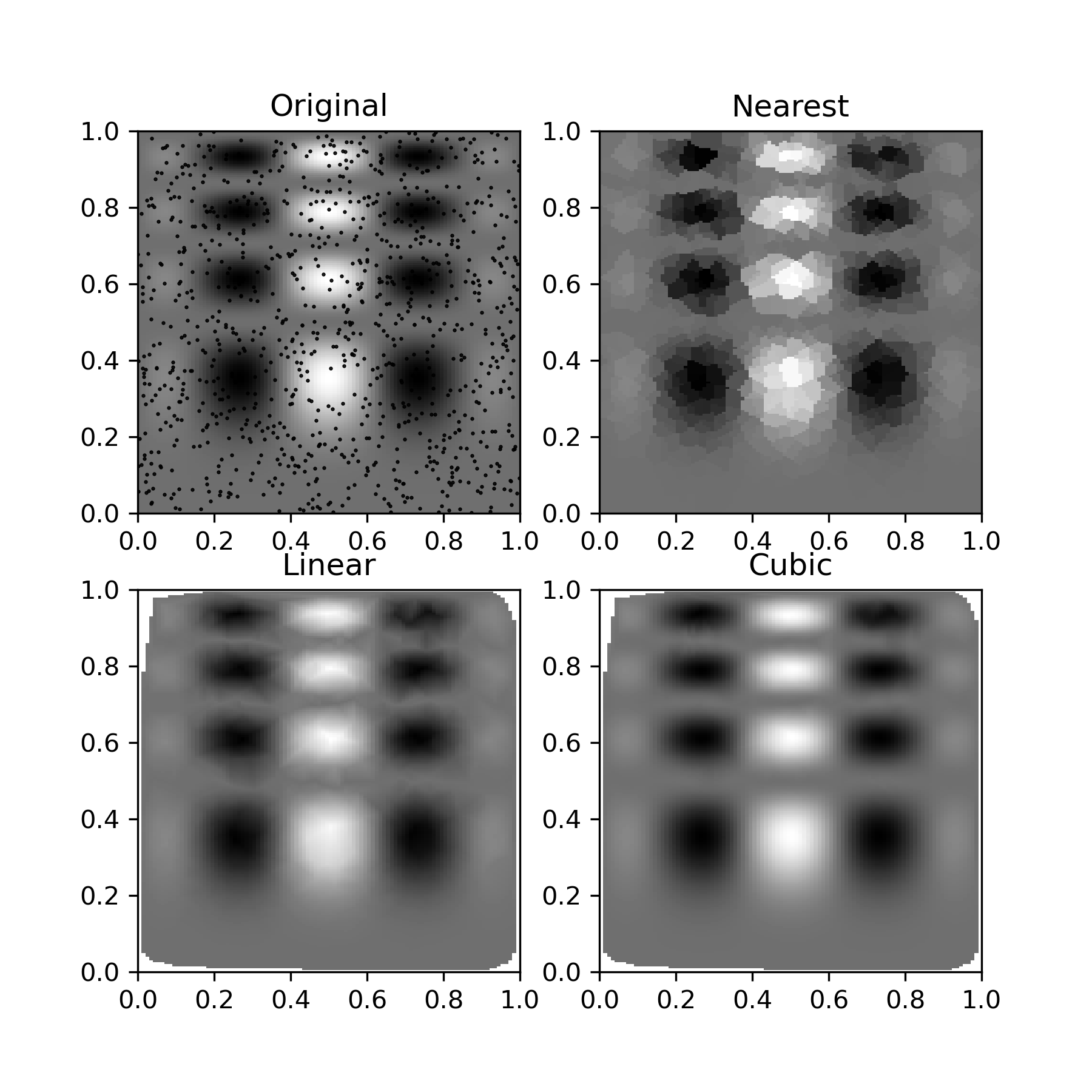
Suppose we want to interpolate the 2-D function
>>> def func(x, y):
...     return x*(1-x)*np.cos(4*np.pi*x) * np.sin(4*np.pi*y**2)**2
on a grid in [0, 1]x[0, 1]
>>> grid_x, grid_y = np.mgrid[0:1:100j, 0:1:200j]
but we only know its values at 1000 data points:
>>> rng = np.random.default_rng()
... points = rng.random((1000, 2))
... values = func(points[:,0], points[:,1])
This can be done with griddata
-- below we try out all of the interpolation methods:
>>> from scipy.interpolate import griddata
... grid_z0 = griddata(points, values, (grid_x, grid_y), method='nearest')
... grid_z1 = griddata(points, values, (grid_x, grid_y), method='linear')
... grid_z2 = griddata(points, values, (grid_x, grid_y), method='cubic')
One can see that the exact result is reproduced by all of the methods to some degree, but for this smooth function the piecewise cubic interpolant gives the best results:
>>> import matplotlib.pyplot as plt
... plt.subplot(221)
... plt.imshow(func(grid_x, grid_y).T, extent=(0,1,0,1), origin='lower')
... plt.plot(points[:,0], points[:,1], 'k.', ms=1)
... plt.title('Original')
... plt.subplot(222)
... plt.imshow(grid_z0.T, extent=(0,1,0,1), origin='lower')
... plt.title('Nearest')
... plt.subplot(223)
... plt.imshow(grid_z1.T, extent=(0,1,0,1), origin='lower')
... plt.title('Linear')
... plt.subplot(224)
... plt.imshow(grid_z2.T, extent=(0,1,0,1), origin='lower')
... plt.title('Cubic')
... plt.gcf().set_size_inches(6, 6)
... plt.show()
The following pages refer to to this document either explicitly or contain code examples using this.
scipy.interpolate._ndgriddata.griddata
scipy.interpolate._ndgriddata.NearestNDInterpolator
scipy.interpolate.interpnd.LinearNDInterpolator
Hover to see nodes names; edges to Self not shown, Caped at 50 nodes.
Using a canvas is more power efficient and can get hundred of nodes ; but does not allow hyperlinks; , arrows or text (beyond on hover)
SVG is more flexible but power hungry; and does not scale well to 50 + nodes.
All aboves nodes referred to, (or are referred from) current nodes; Edges from Self to other have been omitted (or all nodes would be connected to the central node "self" which is not useful). Nodes are colored by the library they belong to, and scaled with the number of references pointing them