solve_bvp(fun, bc, x, y, p=None, S=None, fun_jac=None, bc_jac=None, tol=0.001, max_nodes=1000, verbose=0, bc_tol=None)
This function numerically solves a first order system of ODEs subject to two-point boundary conditions:
dy / dx = f(x, y, p) + S * y / (x - a), a <= x <= b
bc(y(a), y(b), p) = 0
Here x is a 1-D independent variable, y(x) is an N-D vector-valued function and p is a k-D vector of unknown parameters which is to be found along with y(x). For the problem to be determined, there must be n + k boundary conditions, i.e., bc must be an (n + k)-D function.
The last singular term on the right-hand side of the system is optional. It is defined by an n-by-n matrix S, such that the solution must satisfy S y(a) = 0. This condition will be forced during iterations, so it must not contradict boundary conditions. See for the explanation how this term is handled when solving BVPs numerically.
Problems in a complex domain can be solved as well. In this case, y and p are considered to be complex, and f and bc are assumed to be complex-valued functions, but x stays real. Note that f and bc must be complex differentiable (satisfy Cauchy-Riemann equations ), otherwise you should rewrite your problem for real and imaginary parts separately. To solve a problem in a complex domain, pass an initial guess for y with a complex data type (see below).
This function implements a 4th order collocation algorithm with the control of residuals similar to . A collocation system is solved by a damped Newton method with an affine-invariant criterion function as described in .
Note that in integral residuals are defined without normalization by interval lengths. So, their definition is different by a multiplier of h**0.5 (h is an interval length) from the definition used here.
Right-hand side of the system. The calling signature is fun(x, y)
, or fun(x, y, p)
if parameters are present. All arguments are ndarray: x
with shape (m,), y
with shape (n, m), meaning that y[:, i]
corresponds to x[i]
, and p
with shape (k,). The return value must be an array with shape (n, m) and with the same layout as y
.
Function evaluating residuals of the boundary conditions. The calling signature is bc(ya, yb)
, or bc(ya, yb, p)
if parameters are present. All arguments are ndarray: ya
and yb
with shape (n,), and p
with shape (k,). The return value must be an array with shape (n + k,).
Initial mesh. Must be a strictly increasing sequence of real numbers with x[0]=a
and x[-1]=b
.
Initial guess for the function values at the mesh nodes, ith column corresponds to x[i]
. For problems in a complex domain pass y with a complex data type (even if the initial guess is purely real).
Initial guess for the unknown parameters. If None (default), it is assumed that the problem doesn't depend on any parameters.
Matrix defining the singular term. If None (default), the problem is solved without the singular term.
Function computing derivatives of f with respect to y and p. The calling signature is fun_jac(x, y)
, or fun_jac(x, y, p)
if parameters are present. The return must contain 1 or 2 elements in the following order:
Function computing derivatives of bc with respect to ya, yb, and p. The calling signature is bc_jac(ya, yb)
, or bc_jac(ya, yb, p)
if parameters are present. The return must contain 2 or 3 elements in the following order:
Desired tolerance of the solution. If we define r = y' - f(x, y)
, where y is the found solution, then the solver tries to achieve on each mesh interval norm(r / (1 + abs(f)) < tol
, where norm
is estimated in a root mean squared sense (using a numerical quadrature formula). Default is 1e-3.
Maximum allowed number of the mesh nodes. If exceeded, the algorithm terminates. Default is 1000.
Level of algorithm's verbosity:
Desired absolute tolerance for the boundary condition residuals: :None:None:`bc` value should satisfy abs(bc) < bc_tol
component-wise. Equals to :None:None:`tol` by default. Up to 10 iterations are allowed to achieve this tolerance.
Found solution for y as scipy.interpolate.PPoly
instance, a C1 continuous cubic spline.
Found parameters. None, if the parameters were not present in the problem.
Nodes of the final mesh.
Solution values at the mesh nodes.
Solution derivatives at the mesh nodes.
RMS values of the relative residuals over each mesh interval (see the description of :None:None:`tol` parameter).
Number of completed iterations.
Reason for algorithm termination:
0: The algorithm converged to the desired accuracy.
1: The maximum number of mesh nodes is exceeded.
2: A singular Jacobian encountered when solving the collocation system.
Verbal description of the termination reason.
True if the algorithm converged to the desired accuracy ( status=0
).
Solve a boundary value problem for a system of ODEs.
y'' + k * exp(y) = 0 y(0) = y(1) = 0
for k = 1.
y1' = y2 y2' = -exp(y1)
>>> def fun(x, y):
...     return np.vstack((y[1], -np.exp(y[0])))
Implement evaluation of the boundary condition residuals:
>>> def bc(ya, yb):
...     return np.array([ya[0], yb[0]])
Define the initial mesh with 5 nodes:
>>> x = np.linspace(0, 1, 5)
This problem is known to have two solutions. To obtain both of them, we use two different initial guesses for y. We denote them by subscripts a and b.
>>> y_a = np.zeros((2, x.size))
... y_b = np.zeros((2, x.size))
... y_b[0] = 3
Now we are ready to run the solver.
>>> from scipy.integrate import solve_bvp
... res_a = solve_bvp(fun, bc, x, y_a)
... res_b = solve_bvp(fun, bc, x, y_b)
Let's plot the two found solutions. We take an advantage of having the solution in a spline form to produce a smooth plot.
>>> x_plot = np.linspace(0, 1, 100)
... y_plot_a = res_a.sol(x_plot)[0]
... y_plot_b = res_b.sol(x_plot)[0]
... import matplotlib.pyplot as plt
... plt.plot(x_plot, y_plot_a, label='y_a')
... plt.plot(x_plot, y_plot_b, label='y_b')
... plt.legend()
... plt.xlabel("x")
... plt.ylabel("y")
... plt.show()
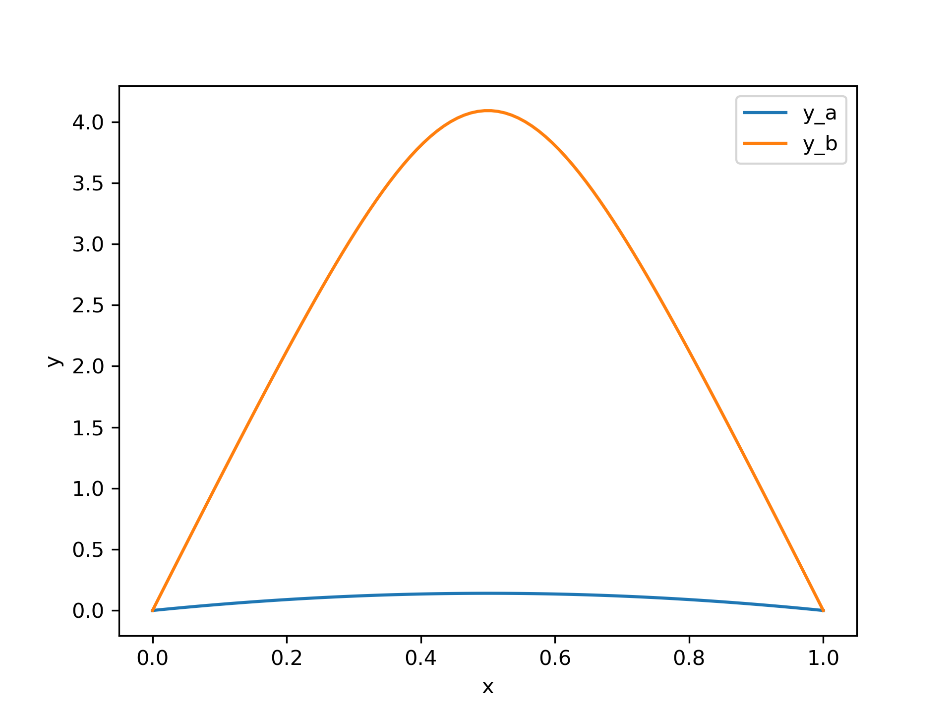
We see that the two solutions have similar shape, but differ in scale significantly.
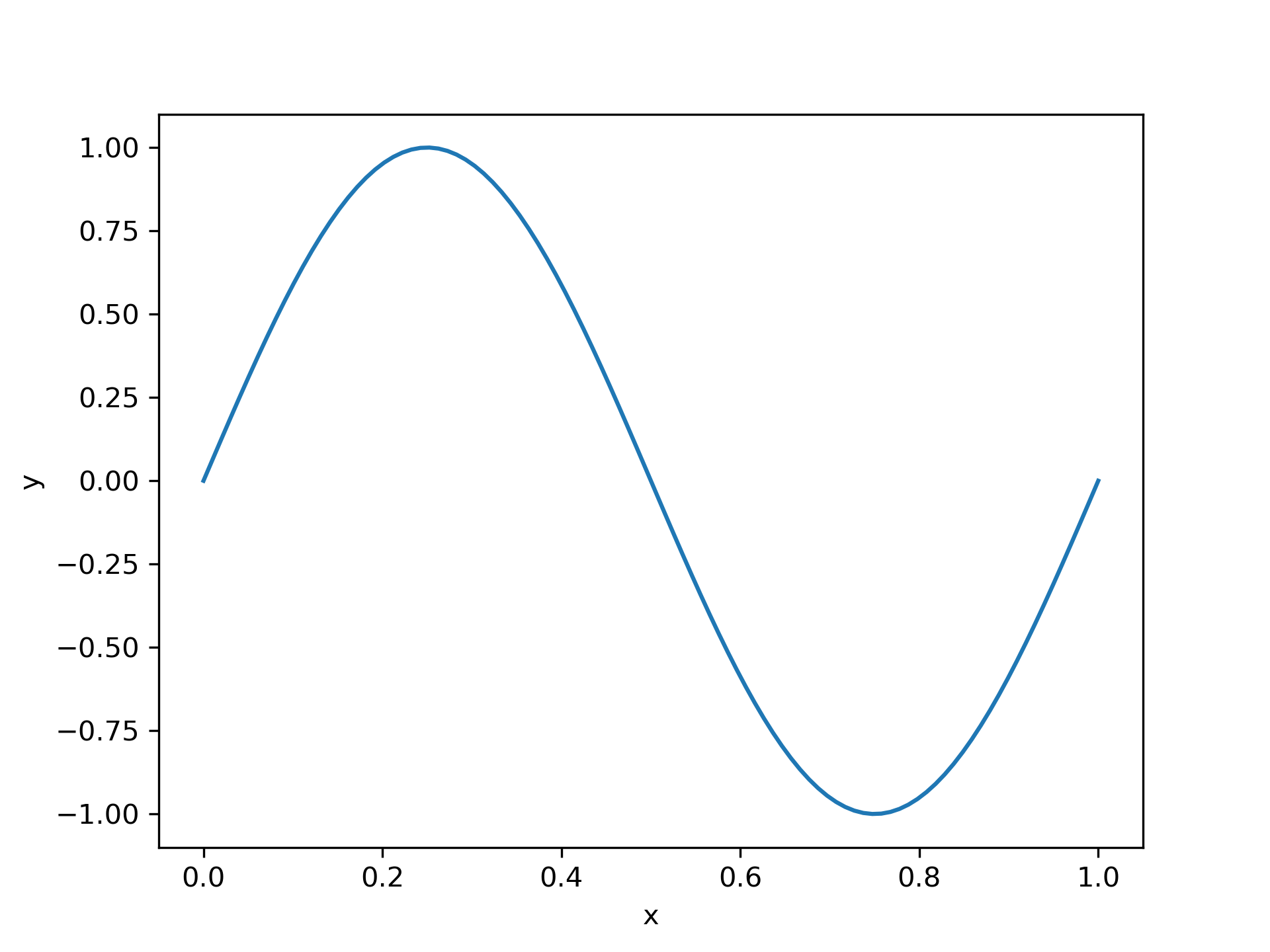
y'' + k**2 * y = 0 y(0) = y(1) = 0
y'(0) = k
y1' = y2 y2' = -k**2 * y1
>>> def fun(x, y, p):
...     k = p[0]
...     return np.vstack((y[1], -k**2 * y[0]))
Note that parameters p are passed as a vector (with one element in our case).
Implement the boundary conditions:
>>> def bc(ya, yb, p):
...     k = p[0]
...     return np.array([ya[0], yb[0], ya[1] - k])
Set up the initial mesh and guess for y. We aim to find the solution for k = 2 * pi, to achieve that we set values of y to approximately follow sin(2 * pi * x):
>>> x = np.linspace(0, 1, 5)
... y = np.zeros((2, x.size))
... y[0, 1] = 1
... y[0, 3] = -1
Run the solver with 6 as an initial guess for k.
>>> sol = solve_bvp(fun, bc, x, y, p=[6])
We see that the found k is approximately correct:
>>> sol.p[0]
6.28329460046
And, finally, plot the solution to see the anticipated sinusoid:
>>> x_plot = np.linspace(0, 1, 100)
... y_plot = sol.sol(x_plot)[0]
... plt.plot(x_plot, y_plot)
... plt.xlabel("x")
... plt.ylabel("y")
... plt.show()
The following pages refer to to this document either explicitly or contain code examples using this.
scipy.integrate._bvp.solve_bvp
Hover to see nodes names; edges to Self not shown, Caped at 50 nodes.
Using a canvas is more power efficient and can get hundred of nodes ; but does not allow hyperlinks; , arrows or text (beyond on hover)
SVG is more flexible but power hungry; and does not scale well to 50 + nodes.
All aboves nodes referred to, (or are referred from) current nodes; Edges from Self to other have been omitted (or all nodes would be connected to the central node "self" which is not useful). Nodes are colored by the library they belong to, and scaled with the number of references pointing them