fft(a, n=None, axis=-1, norm=None)
This function computes the one-dimensional n-point discrete Fourier Transform (DFT) with the efficient Fast Fourier Transform (FFT) algorithm [CT].
FFT (Fast Fourier Transform) refers to a way the discrete Fourier Transform (DFT) can be calculated efficiently, by using symmetries in the calculated terms. The symmetry is highest when n is a power of 2, and the transform is therefore most efficient for these sizes.
The DFT is defined, with the conventions used in this implementation, in the documentation for the numpy.fft
module.
Input array, can be complex.
Length of the transformed axis of the output. If n is smaller than the length of the input, the input is cropped. If it is larger, the input is padded with zeros. If n is not given, the length of the input along the axis specified by :None:None:`axis` is used.
Axis over which to compute the FFT. If not given, the last axis is used.
Normalization mode (see numpy.fft
). Default is "backward". Indicates which direction of the forward/backward pair of transforms is scaled and with what normalization factor.
The "backward", "forward" values were added.
If :None:None:`axis` is not a valid axis of a.
The truncated or zero-padded input, transformed along the axis indicated by :None:None:`axis`, or the last one if :None:None:`axis` is not specified.
Compute the one-dimensional discrete Fourier Transform.
fft2
The two-dimensional FFT.
fftfreq
Frequency bins for given FFT parameters.
fftn
The n-dimensional FFT.
ifft
The inverse of :None:None:`fft`.
numpy.fft
for definition of the DFT and conventions used.
rfftn
The n-dimensional FFT of real input.
>>> np.fft.fft(np.exp(2j * np.pi * np.arange(8) / 8))
array([-2.33486982e-16+1.14423775e-17j,  8.00000000e+00-1.25557246e-15j,
        2.33486982e-16+2.33486982e-16j,  0.00000000e+00+1.22464680e-16j,
       -1.14423775e-17+2.33486982e-16j,  0.00000000e+00+5.20784380e-16j,
        1.14423775e-17+1.14423775e-17j,  0.00000000e+00+1.22464680e-16j])
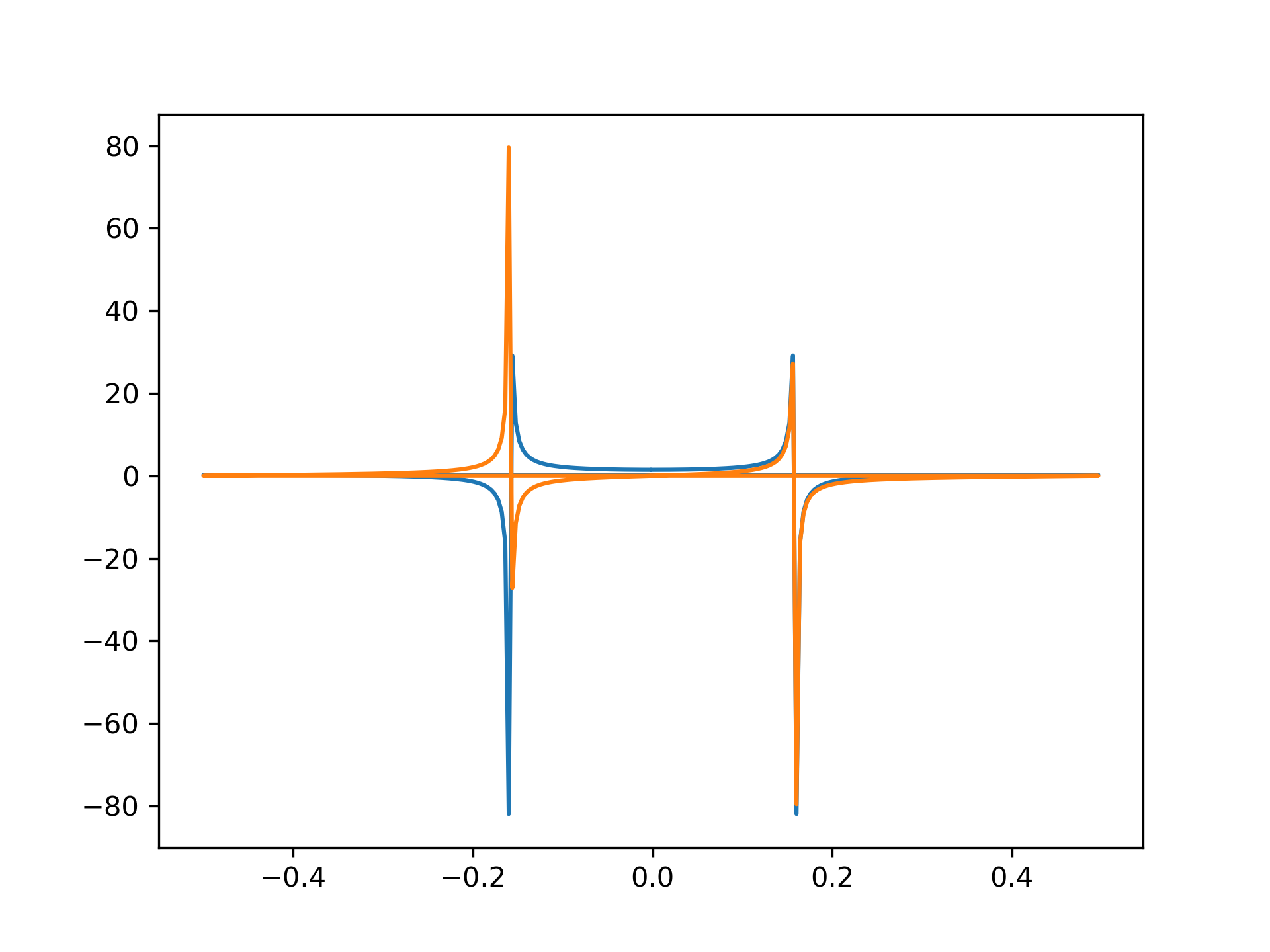
In this example, real input has an FFT which is Hermitian, i.e., symmetric in the real part and anti-symmetric in the imaginary part, as described in the numpy.fft
documentation:
>>> import matplotlib.pyplot as plt
... t = np.arange(256)
... sp = np.fft.fft(np.sin(t))
... freq = np.fft.fftfreq(t.shape[-1])
... plt.plot(freq, sp.real, freq, sp.imag)
[<matplotlib.lines.Line2D object at 0x...>, <matplotlib.lines.Line2D object at 0x...>]
>>> plt.show()
The following pages refer to to this document either explicitly or contain code examples using this.
dask.array.fft.fft_wrap
scipy.special._basic.diric
dask.array.fft.fftfreq
Hover to see nodes names; edges to Self not shown, Caped at 50 nodes.
Using a canvas is more power efficient and can get hundred of nodes ; but does not allow hyperlinks; , arrows or text (beyond on hover)
SVG is more flexible but power hungry; and does not scale well to 50 + nodes.
All aboves nodes referred to, (or are referred from) current nodes; Edges from Self to other have been omitted (or all nodes would be connected to the central node "self" which is not useful). Nodes are colored by the library they belong to, and scaled with the number of references pointing them