>>> """
=====================
Time Series Histogram
=====================

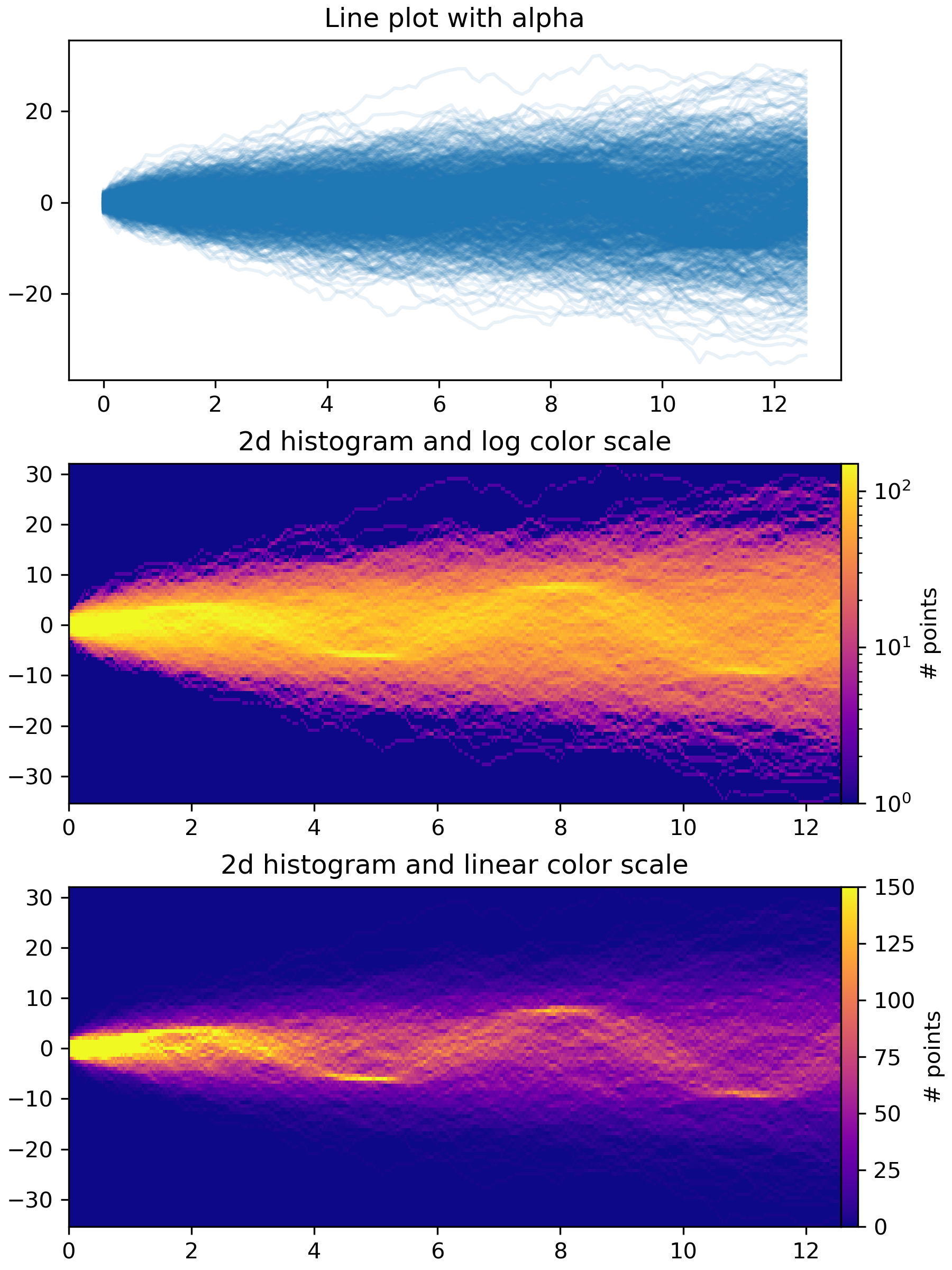
This example demonstrates how to efficiently visualize large numbers of time
series in a way that could potentially reveal hidden substructure and patterns
that are not immediately obvious, and display them in a visually appealing way.

In this example, we generate multiple sinusoidal "signal" series that are
buried under a larger number of random walk "noise/background" series. For an
unbiased Gaussian random walk with standard deviation of σ, the RMS deviation
from the origin after n steps is σ*sqrt(n). So in order to keep the sinusoids
visible on the same scale as the random walks, we scale the amplitude by the
random walk RMS. In addition, we also introduce a small random offset ``phi``
to shift the sines left/right, and some additive random noise to shift
individual data points up/down to make the signal a bit more "realistic" (you
wouldn't expect a perfect sine wave to appear in your data).

The first plot shows the typical way of visualizing multiple time series by
overlaying them on top of each other with ``plt.plot`` and a small value of
``alpha``. The second and third plots show how to reinterpret the data as a 2d
histogram, with optional interpolation between data points, by using
``np.histogram2d`` and ``plt.pcolormesh``.
"""
... from copy import copy
... import time
... 
... import numpy as np
... import numpy.matlib
... import matplotlib.pyplot as plt
... from matplotlib.colors import LogNorm
... 
... fig, axes = plt.subplots(nrows=3, figsize=(6, 8), constrained_layout=True)
... 
... # Make some data; a 1D random walk + small fraction of sine waves
... num_series = 1000
... num_points = 100
... SNR = 0.10  # Signal to Noise Ratio
... x = np.linspace(0, 4 * np.pi, num_points)
... # Generate unbiased Gaussian random walks
... Y = np.cumsum(np.random.randn(num_series, num_points), axis=-1)
... # Generate sinusoidal signals
... num_signal = int(round(SNR * num_series))
... phi = (np.pi / 8) * np.random.randn(num_signal, 1)  # small random offset
... Y[-num_signal:] = (
...     np.sqrt(np.arange(num_points))[None, :]  # random walk RMS scaling factor
...     * (np.sin(x[None, :] - phi)
...        + 0.05 * np.random.randn(num_signal, num_points))  # small random noise
... )
... 
... 
... # Plot series using `plot` and a small value of `alpha`. With this view it is
... # very difficult to observe the sinusoidal behavior because of how many
... # overlapping series there are. It also takes a bit of time to run because so
... # many individual artists need to be generated.
... tic = time.time()
... axes[0].plot(x, Y.T, color="C0", alpha=0.1)
... toc = time.time()
... axes[0].set_title("Line plot with alpha")
... print(f"{toc-tic:.3f} sec. elapsed")
... 
... 
... # Now we will convert the multiple time series into a histogram. Not only will
... # the hidden signal be more visible, but it is also a much quicker procedure.
... tic = time.time()
... # Linearly interpolate between the points in each time series
... num_fine = 800
... x_fine = np.linspace(x.min(), x.max(), num_fine)
... y_fine = np.empty((num_series, num_fine), dtype=float)
... for i in range(num_series):
...     y_fine[i, :] = np.interp(x_fine, x, Y[i, :])
... y_fine = y_fine.flatten()
... x_fine = np.matlib.repmat(x_fine, num_series, 1).flatten()
... 
... 
... # Plot (x, y) points in 2d histogram with log colorscale
... # It is pretty evident that there is some kind of structure under the noise
... # You can tune vmax to make signal more visible
... cmap = copy(plt.cm.plasma)
... cmap.set_bad(cmap(0))
... h, xedges, yedges = np.histogram2d(x_fine, y_fine, bins=[400, 100])
... pcm = axes[1].pcolormesh(xedges, yedges, h.T, cmap=cmap,
...                          norm=LogNorm(vmax=1.5e2), rasterized=True)
... fig.colorbar(pcm, ax=axes[1], label="# points", pad=0)
... axes[1].set_title("2d histogram and log color scale")
... 
... # Same data but on linear color scale
... pcm = axes[2].pcolormesh(xedges, yedges, h.T, cmap=cmap,
...                          vmax=1.5e2, rasterized=True)
... fig.colorbar(pcm, ax=axes[2], label="# points", pad=0)
... axes[2].set_title("2d histogram and linear color scale")
... 
... toc = time.time()
... print(f"{toc-tic:.3f} sec. elapsed")
... plt.show()
... 
... #############################################################################
... #
... # .. admonition:: References
... #
... #    The use of the following functions, methods, classes and modules is shown
... #    in this example:
... #
... #    - `matplotlib.axes.Axes.pcolormesh` / `matplotlib.pyplot.pcolormesh`
... #    - `matplotlib.figure.Figure.colorbar`
...